ML Beginner's Guide to Build Car Damage Detection AI Model

The problem of vehicle damage plagues the automotive industry. Vehicles are prone to damage in several ways, including accidents, collisions, natural disasters, and wear and tear. This problem affects several industries, including car manufacturers, insurers, car rental companies, and individual vehicle owners.

The insurance industry needs to quickly and accurately assess the extent of damage to vehicles involved in accidents to process claims.

The problem is significant, as inaccurate or delayed damage assessments can lead to increased costs for insurers, longer processing times for claims, and customer dissatisfaction. According to industry estimates, auto insurance claims can take ten days to process, costing $4,000 per claim. Inaccurate assessments can also lead to fraud, which costs the industry billions of dollars annually.

             Figure: Damaged vehicle

In addition to the cost of repairs, vehicle damage can result in other losses, such as lost productivity due to downtime, increased insurance premiums, and reduced resale value.

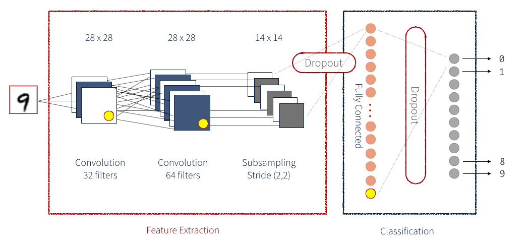
         Figure: Overview of vehicle damage detection

Computer vision technology can play a significant role in solving the problem of vehicle damage. Using machine learning algorithms, computer vision systems can quickly and accurately identify vehicle damage, including dents, scratches, and other types of damage.

One such company which utilizes computer vision to solve the problem of vehicle damage detection is Tractable.

Tractable is an AI-driven company specializing in computer vision solutions for the insurance industry. They use advanced algorithms to automate and improve processes such as vehicle damage assessment, estimation of repair costs, and claims processing.

By streamlining these processes, Tractable helps insurers to process claims more efficiently and accurately, improving customer satisfaction and reducing costs.

Tractable uses computer vision technology to automate the process of vehicle damage detection and estimation. Below are some tasks:

1. Image capture: The first step is to capture images of the damaged vehicle using a smartphone, tablet, or another device.
2. Image processing: Once the images are captured, they are uploaded to Tractable's cloud-based platform, which computer vision algorithms process.
3. Damage estimation: Based on the analysis of the images, Tractable's system estimates the repair cost.
4. Claims processing: The insurance company then uses the estimated repair cost to process the claim.

Prerequisites

To proceed further and understand CNN based approach for detecting casting defects, one should be familiar with the following:

1. Python: We will be using Python for the below tutorial.
2. Tensorflow: TensorFlow is a free, open-source machine learning and artificial intelligence software library. It can be utilized for various tasks but is most commonly employed for deep neural network training and inference.
3. Keras: Keras is a Python interface for artificial neural networks and is open-source software. Keras serves as an interface for the TensorFlow library.
4. Kaggle: Kaggle is a platform for data science competitions where users can work on real-world problems, build their skills, and compete with other data scientists. It also provides a community for sharing and collaborating on data science projects and resources.

Apart from the above-listed tools, there are certain other theoretical concepts one should be familiar with to understand the below tutorial.

Transfer Learning

Transfer learning is a machine learning technique that adapts a pre-trained model to a new task. This technique is widely used in deep learning because it dramatically reduces the data and computing resources required to train a model.

This technique avoids the need to start the training process from scratch, as it takes advantage of the knowledge learned from solving the first problem that has already been trained on a large dataset.

The pre-trained model can be a general-purpose model trained on a large dataset like ImageNet or a specific model trained for a similar task. The idea behind transfer learning is that the learned features in the pre-trained model are highly relevant to the new task and can be used as a starting point for fine-tuning the model on the new dataset.

Transfer learning has proven highly effective in various applications, including computer vision, natural language processing, and speech recognition.

Binary Cross Entropy function

Binary cross entropy loss is a loss function used in binary classification tasks, where the goal is to predict a binary output (e.g., true/false, 0/1). It measures the difference between the predicted probability distribution and the actual probability distribution of the output. Mathematically, it is defined as

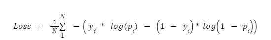
Here, yi is the true probability, and pi is the model's predicted probability.

Methodology

To proceed with our vehicle damage detection system:

1. We begin by importing the required libraries.
2. Next, we preprocess our data, which includes resizing our images, one-hot encoding our labels, etc.
3. Creating the model is done by adding new layers to a pre-trained model.
4. Training the model on the dataset.
5. Plotting and visualizing the output.

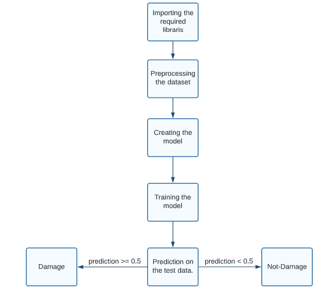
                        Figure: Flowchart for methodology

Dataset Selection

For this tutorial, we have used the dataset available at Kaggle. The dataset contains a total of 1610 images, out of which 1150 training images and 460 validation images. The dataset is arranged in such a manner:

1. We first have two folders, training and validation.
2. In each folder, we again have two folders, 00-damage and 01-whole.

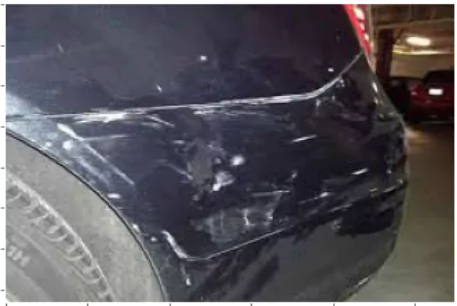
     Figure: Damaged Vehicle

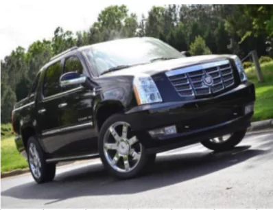
    Figure: Not-Damaged Vehicle

The images used are 3-channel RGB images with a size of (480, 640, 3).

Large-scale annotation and categorization of data can be facilitated by the effective data labeling platform Labellerr. Users can design labeling tasks, invite colleagues, and employ machine learning models to automate and expedite the labeling process using its user-friendly interface.

Text, images, and videos are just a few of the many data formats that Labellerr supports and a vast variety of annotation techniques it offers. In addition, it supports task management, collaboration, and quality control, making it a useful tool for data labeling requirements. Contact us right away!

Implementation

The below points are to be noted before starting the tutorial.

1. The below code is written in my Kaggle notebook. For this, you first need to have a Kaggle account. So, if not, you need to sign up and create a Kaggle account.
2. Once you have created your account, visit Vehicle damage detection and create a new notebook.
3. Run the below code as given. For better results, you can further try hyperparameter tuning, i.e., try to change the batch size, number of epochs, etc.

Hands-on with Code

We begin by importing the required libraries.

# import the necessary libraries

# For data augmentation while data preprocessing
from tensorflow.keras.preprocessing.image import ImageDataGenerator

# Pretrained MobileNet model.
from tensorflow.keras.applications import MobileNetV2

# Performing MaxPooling operations
from tensorflow.keras.layers import MaxPooling2D

# For performing dropout operation
from tensorflow.keras.layers import Dropout

# For flattening operation
from tensorflow.keras.layers import Flatten
from tensorflow.keras.layers import Dense

# Input() is used to instantiate a Keras tensor.
from tensorflow.keras.layers import Input
from tensorflow.keras.models import Model

# We use adam optimizer
from tensorflow.keras.optimizers import Adam

# Preprocesses a tensor or Numpy array encoding a batch of images.
from tensorflow.keras.applications.mobilenet_v2 import preprocess_input

# Converts a PIL Image instance to a Numpy array.
from tensorflow.keras.preprocessing.image import img_to_array

# Loads an image into PIL format.
from tensorflow.keras.preprocessing.image import load_img

# Converts a class vector (integers) to binary class matrix.
from tensorflow.keras.utils import to_categorical

# Binarize labels in a one-vs-all fashion.
from sklearn.preprocessing import LabelBinarizer

# Performing train-test split
from sklearn.model_selection import train_test_split

# For printing the metrics
from sklearn.metrics import classification_report

# For using strings in file structure path format
from imutils import paths

# For plotting losse functions
import matplotlib.pyplot as plt

# For performing mathematical computations
import numpy as np

# For file-related operations
import os

Next, we perform some data visualization to understand the data. It means we compute specific statistical parameters on our data along with its visualization.

# Path to directory containing data
DataDir = "/kaggle/input/car-damage-detection/data1a"

# Path to training directory
train_dir = os.path.join(DataDir, 'training/')

# Path to validation directory
val_dir = os.path.join(DataDir, 'validation/')

# Path for damaged training images
train_damage = os.path.join(train_dir, '00-damage')
# Path for training images not damaged
train_not_damage = os.path.join(val_dir, '01-whole')

# Number of damaged training images
num_train_damage = len(os.listdir(train_damage))

# Number of training images not damaged
num_train_not_damage = len(os.listdir(train_not_damage))

# Path for damaged validation
val_damage = os.path.join(val_dir, '00-damage')

# Path for validation images not damaged
val_not_damage = os.path.join(val_dir, '01-whole')

# Number of damaged validation images
num_val_damage = len(os.listdir(val_damage))

# Number of validation images not damaged
num_val_not_damage = len(os.listdir((val_not_damage)))

# Number of training images
num_train = num_train_damage + num_train_not_damage

# Number of validation images
num_val = num_val_damage + num_val_not_damage


# Total images
total_images = num_val + num_train
print("Total training images",num_train)
print("Total training images (Damaged)", num_train_damage)
print("Total training images (Damaged)", num_train_not_damage)
print()

print("Total validation images", num_val)
print("Total training images (Damaged)", num_val_damage)
print("Total training images (Damaged)", num_val_not_damage)
print()

print("Total Number of Images: ",total_images)

# Plotting a sample image
plt.grid('')
image = plt.imread('/kaggle/input/car-damage-detection/data1a/training/01-whole/0195.jpg')
plt.imshow(image)
plt.show()

Next, we set our initial hyperparameters. This includes the learning rate, number of epochs, and batch size. We also set up a class vector containing two classes:

1. Damaged (00-damage)
2. Not-damaged (01-whole)

# initializing the hyperparameters
initial_lr = 0.001
epochs = 100
batch_size = 64

# Classes which are detected
classes = ["00-damage", "01-whole"]

Why is the batch size chosen to be 64?

One reason for setting the batch size to 64 is that it balances the benefits of using large and small batch sizes.

With a small batch size, such as 1, the model can update its weights after each example, resulting in faster convergence. However, small batch sizes may not fully utilize the computational resources available and can result in higher variability in the updates.

On the other hand, a large batch size, such as 1024, can efficiently utilize computational resources and lead to more stable updates. However, large batch sizes may require more memory and can slow down the convergence.

A batch size of 64 balances these two approaches, allowing for efficient use of the computational resources while still allowing for fast convergence and stable updates. Additionally, a batch size of 64 is a common choice in deep learning because it works well with modern hardware, such as GPUs, which are optimized for processing batches of data in parallel.

Next, we do some data preprocessing. This includes

1. Creating an array of data and labels stores the data and its corresponding labels from the dataset directory.
2. Doing the train-test split on the data.
3. Perform some data augmentation on the images. This is used to generalize the model over the data well. For this purpose:

1. width_shift_range and height_shift_range: specify the range (as a fraction of the total image width or height) of random horizontal and vertical shifts that can be applied to the images.
2. Zoom range: specifies the range of random zooms that can be used to image
3. Random rotations: specifies the range (in degrees) of random rotations that can be applied to the images.
4. Horizontal_flip: specifies whether or not to flip images horizontally randomly.
5. flip_mode: specifies the method used to fill in pixels created by the transformations (e.g., "nearest" fills in new pixels with the value of the nearest pixel in the original image).

# grab the list of images in our dataset directory, then initialize
# the list of data (i.e., images) and class images
print("[INFO] loading images...")

# It stores the data or feature set
data = []

# It stores the corrosponding labels
labels = []

for class_ in classes:
    path = os.path.join(train_dir, class_)
    for image in os.listdir(path):
    	image_path = os.path.join(path, image)
    	image_ = load_img(image_path, target_size=(224, 224))
    	image_ = img_to_array(image_)
    	image_ = preprocess_input(image_)

    	data.append(image_)
    	labels.append(class_)


for class_ in classes:
    path = os.path.join(val_dir, class_)
    for image in os.listdir(path):
    	image_path = os.path.join(path, image)
    	image_ = load_img(image_path, target_size=(224, 224))
    	image_ = img_to_array(image_)
    	image_ = preprocess_input(image_)

    	data.append(image_)
    	labels.append(class_)
        
# perform one-hot encoding on the labels
lb = LabelBinarizer()
labels = lb.fit_transform(labels)
labels = to_categorical(labels)

data = np.array(data, dtype="float32")
labels = np.array(labels)



(trainX, testX, trainY, testY) = train_test_split(data, labels,
	test_size=0.20, stratify=labels, random_state=42)

# construct the training image generator for data augmentation
aug = ImageDataGenerator(
	rotation_range=20,
	zoom_range=0.15,
	width_shift_range=0.2,
	height_shift_range=0.2,
	shear_range=0.15,
	horizontal_flip=True,
	fill_mode="nearest")

After data preprocessing, we now create our model. We use a pre-trained mobile net architecture without the top layer, which can be used as a feature extractor for transfer learning.

Using a pre-trained model as a base, we can leverage the knowledge learned by the MobileNetV2 model on a large dataset and adapt it to a new task with a smaller dataset.

# loading the MobileNetV2 network, ensuring the topmost fully-connected
# layer sets are left off
model_base = MobileNetV2(weights="imagenet", include_top=False,
	input_tensor=Input(shape=(224, 224, 3)))

# Constructing the top architecture of our model, which is placed over the 
# pretrained model
model_head = model_base.output
# MaxPooling layer

model_head = MaxPooling2D(pool_size=(5, 5))(model_head)
# Flatten layer
model_head = Flatten(name="flatten")(model_head)

# Activation function relu
model_head = Dense(128, activation="relu")(model_head)

# Performing dropout
model_head = Dropout(0.5)(model_head)

# Final output layer consists of softmax layer
model_head = Dense(2, activation="softmax")(model_head)

# place the head FC model on top of the base model (this will become
# the actual model we will train)
model_final = Model(inputs=model_base.input, outputs=model_head)

Why is MobileNet architecture used?

MobileNet architecture is used because it is lightweight, efficient, and optimized for mobile and embedded devices. It allows for real-time object detection and classification while keeping the computational and memory requirements low, making it an ideal choice for computer vision applications in mobile and embedded devices.

As we have only to train the top layers of our model, we make the trainability of other layers of the base model false.

# looping over all the layers and setting each individual layer trainability
# to false.
for layer in model_base.layers:
	layer.trainable = False

Next, we set our model's optimizer function and compiled it. When compiling:

1. We set the loss function to binary_cross_entropy
2. Optimizer to Adam
3. Evaluation metric to accuracy

# Setting optimizer to Adam 
optim = Adam(lr=initial_lr, decay=initial_lr / epochs)

# Compiling our model
model_final.compile(loss="binary_crossentropy", optimizer=optim,
	metrics=["accuracy"])

Now, we train our model.

# train the head of the network
model_train = model_final.fit(
#     Generates image generator from ImageGeneratorClass for inputing images in batches
	aug.flow(trainX, trainY, batch_size=batch_size),
#     Number of steps to be taken in one epoch over image batches
	steps_per_epoch=len(trainX) // batch_size,
#     Validation data
	validation_data=(testX, testY),
    
#     Steps for validation data
	validation_steps=len(testX) // batch_size,
    
#     Number of epochs
	epochs=epochs)

Finally, we perform inference on the test set. After prediction, we print the whole classification report to display various evaluation metrics. Also, we save our model as a checkpoint.

# Now, we predict on test set.
predict = model_final.predict(testX, batch_size=batch_size)

# for each image in the test set we find the index of the
# label with corresponding largest predicted probability
predict_index = np.argmax(predict, axis=1)

# Displaying classification report
print(classification_report(testY.argmax(axis=1), predict_index,
	target_names=lb.classes_))

# Storing our model for further use.
model_final.save("Car_detection.model", save_format="h5")

Output

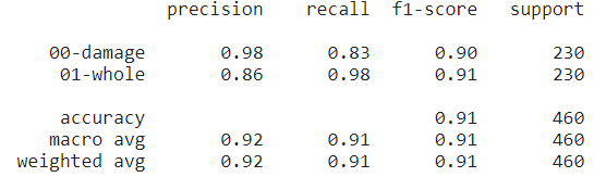
       Figure: Model's classification report

From the above, we can see that an accuracy of 91% is achieved on the test set. This indicates that, out of 100, we have 91 times correct predictions of whether a vehicle is damaged.

In the end, we plot

1. Train Loss vs. Validation Loss
2. Train Accuracy vs. Validation Accuracy

for a better understanding of our model.

# plotting training loss and accuracy
num = epochs

# matplotlib style
plt.style.use("seaborn")
plt.figure()

# Plotting all the required quantities
# Train Accuracy
plt.plot(np.arange(0, num), model_train.history["accuracy"], label="Train Accuracy")

# Validation Accuracy
plt.plot(np.arange(0, num), model_train.history["val_accuracy"], label="Validation Accuracy")

# Train Loss
plt.plot(np.arange(0, num), model_train.history["loss"], label="Train Loss")

# Validation Loss
plt.plot(np.arange(0, num), model_train.history["val_loss"], label="Validation Loss")

# Setting the title
plt.title("Training Loss and Accuracy")

# Setting the label
plt.xlabel("Epochs")
plt.ylabel("Accuracy/Loss")
plt.legend(loc="upper right")

# Saving the Model
plt.savefig("Car_Detection.png")

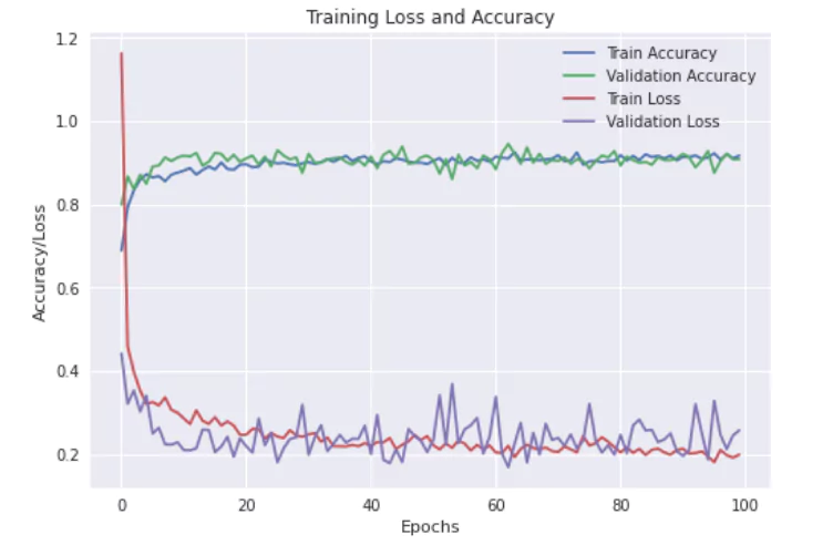
            Figure: Loss and Accuracy plot

From the above plot, we can see that the loss function and accuracy have a lot of oscillations while converging to their respective values. It indicates that the learning rate may be higher than it should be.

Thus, you can tune the learning rate and train the model to achieve better accuracy and performance. For instance, we have used a learning rate of 0.01. We can try training it with some lower learning rates and longer epochs.

This can be achieved using hyper-parameter tuning.

Conclusion

In this blog, we have built a vehicle damage system that uses computer vision and deep learning Methodology to detect by using input images of the vehicle. Big firms and companies like Tractable and Nauto have built large-scale solutions using these vehicle damage detection techniques.

In the above blog, we have built a prototype for a vehicle detection system. Below are the important points:

1. We begin by analyzing our dataset. The dataset in total contains 1610 images of damaged and non-damaged vehicles images.
2. Next, we perform some data augmentation to generalize our model better. This helps prevent overtraining the model.
3. We created our model. Here, we used a pre-trained Mobilenet architecture, which is used as a base model. We built a two-layer architecture over our base model.
4. Next, we trained our model.
5. Finally, in the end, we performed predictions on test images.
6. We achieved an accuracy of 93 percent with 100 epochs. We can increase the number of epochs to achieve greater accuracy.

Looking for high quality training data to train your car damage detection model? Talk to our team to get a tool demo.