Math behind GAN (generative adversarial networks) & its applications

A generative model G and a discriminative model D make up the Generative Adversarial Network (GAN). The discriminative model is comparable to the police seeking to seize counterfeit money, but the generative model might be compared to a forger trying to create phony money and utilize it without being discovered. This competition continues until the counterfeiter develops the intelligence necessary to effectively deceive the cops. Get to know about the math behind the GAN and its application in this blog in detail.

What is GAN?

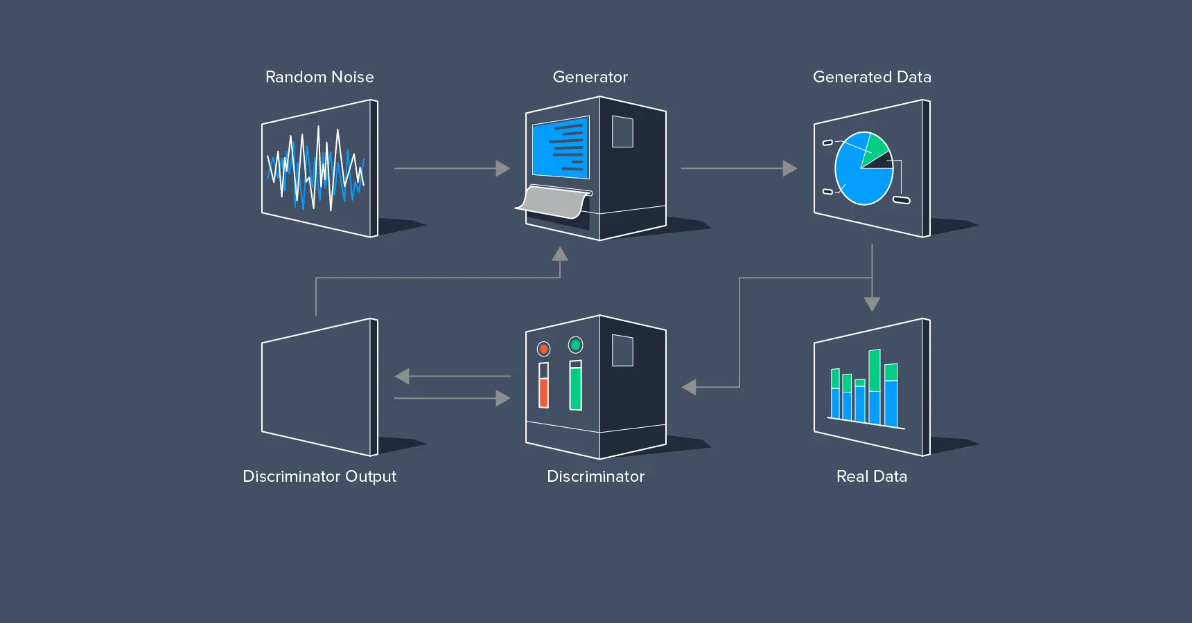
In a generative adversarial network (GAN), two neural networks compete with one another to make predictions that are as accurate as possible. GANs typically operate unsupervised and learn through cooperative zero-sum games.

The generator and the discriminator are the two neural networks that constitute a GAN (generative adversarial network). A de-convolutional neural network serves as the discriminator, and a convolutional neural network serves as the generator. The generator's objective is to provide outputs that could be mistaken for actual data by users. The discriminator's objective is to determine whether the outputs it receives were produced intentionally.

Read about GAN and its working  in detail:

GAN Most Popular Applications

GANs are gaining popularity as a suitable ML model for online retail sales due to their significant improvement in understanding and recreating visual content.

Among the recently identified applications for GANs are:

Security: Although artificial intelligence has benefited numerous businesses, it is also plagued by the issue of cyber threats.

GANs have shown to be quite useful in defending against hostile attacks. The adversarial attacks deceive deep learning architectures using a number of strategies. We defend against these attacks by building phony examples and teaching the model to spot them.

Creating Data with GANs: The most crucial component of every deep learning system is data. Any algorithm using deep learning will perform better in general the more data it has. However, there is a requirement to provide high-quality data in many situations where the volume of data is constrained, such as in medical diagnostics. for what purposes GANs are employed.

• Completing pictures with an outline.
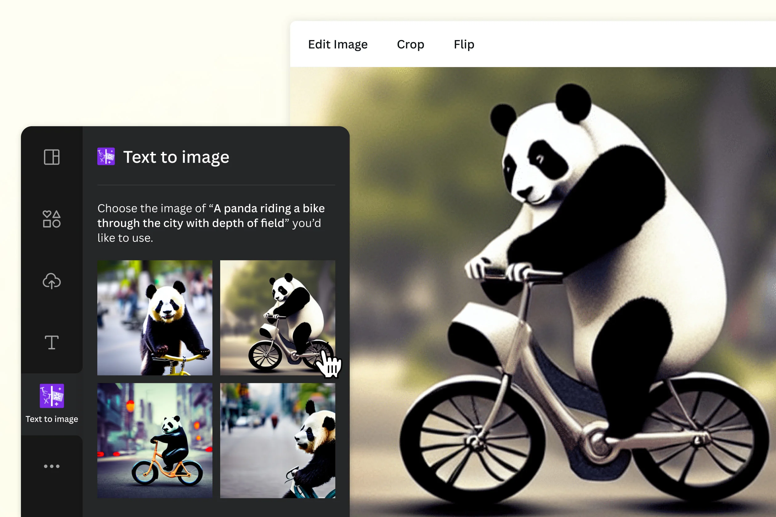
• Creating a credible picture from text.
• Ex-DALL-E: A recently developed deep learning network by openai, also performs text-to-image synthesis. Although the architecture uses a GPT-3 variant rather than GANs.
• Text-to-image creation

StackedGAN

Images can be created using Stacked Generative Adversarial Networks (StackGAN), which are conditioned on text descriptions.

The architecture consists of several stacked GAN models for both text and images. The conditional GAN class is once more involved. There are two GANs in it, also referred to as stage-I and stage-II GANs. In the sketch-refinement method used by StackGAN, the Stage-I GAN, the first level generator, is conditioned on text and produces a low-resolution image, i.e. the simple shape and colors of the descriptive text.

The low-resolution image and the text are both used to condition the Stage-II GAN, which builds on the Stage-I results by adding enticing detail.

• Creating images of photo realistic product prototypes.
• Bringing color to black and white images.

Maintaining Privacy: There are numerous situations where the privacy of our data is required. This is especially helpful for military and defense applications. Although there are various data encryption methods available, each has drawbacks. In these situations, GANs can be helpful. In 2016, Google unveiled a new research direction on the use of the GAN competitive framework for encryption challenges, in which two networks competed to create and decipher the code.

Data manipulation: GANs can be used to edit a portion of the subject without completely transferring the style. In many situations, for instance, users would like to add a smirk to an image or focus only on the image's eyes. This can also be applied to other fields like speech recognition and natural language processing. For instance, we can change a few words in a paragraph without changing the entire text.

GANs can be applied in video production to:

• Model movement and behavior patterns of people inside a frame.
• project future frames of the video.
• Make a deep fake

GANs are frequently used in a variety of industries and for a wide range of challenges. They appear to be simple to train, but in reality, doing so needs two networks, which makes them unstable.

Math Behind Generative adversarial network

The Loss Function's Motivation Permalink

The generator and discriminator are two separate models that interact to form the GAN. As a result, every model will have a unique loss function. Let's try to encourage an intuitive knowledge of the loss function for each in this section.

Let's describe a few parameters and variables before we start the derivation.

• x:Real data
• z:Latent vector
• G(z):Fake data
• D(x):Discriminator's evaluation of real data
• D(G(z)):Discriminator's evaluation of fake data
• Error(a,b):Error between a and b

The Discriminator

The discriminator's objective is to accurately classify produced images as false and empirical data sets as true. Therefore, we may consider the following to represent the loss function of the discriminator:

LD=Error(D(x),1)+Error(D(G(z)),0)--(1)

Here, we refer to a function that tells us the separation or difference between the two functional parameters as Error by utilizing a very general, non-specific notation. (You are definitely on the right track if this made you think of something like cross entropy or Kullback-Leibler divergence).

The Generator

The discriminator must be as perplexed as possible for the generator to succeed in mislabeling produced images as real.

LG=Error(D(G(z)),1)---(2)

Here, it's important to keep in mind that we want to minimize a loss function. The generator should make an effort to reduce the discrepancy between label 1, the label for actual data, and the discriminator's assessment of the generated phone data.

Binary cross entropy

Binary cross entropy is a frequent loss function in binary classification issues. Let's quickly review the cross entropy formula, which is as follows:

H(p,q)=Ex∼p(x)[−logq(x)]--(3)

The random variable in classification problems is discrete. So, the anticipation can be described as a sum.

H(p,q)=−∑x∈χp(x)logq(x)--(4)

In the instance of binary cross entropy, there are about two labels: zero and one, therefore we can further reduce this calculation.

H(y,y^)=−∑y log(y^)+(1−y)log(1−y^)--(5)

The Error function that we ad hoc used in the sections above is this one. In measuring how dissimilar two distributions are in the context of binary classification—which determines whether an input data point is true or false—binary cross entropy achieves our goal. If this is used with the loss functions in (1),

LD=−∑x∈χ,z∈ζlog(D(x))+log(1−D(G(z)))--(6)

The same applies to (2):

Now that we have two loss functions, we can train both the discriminator and the generator using them. Because log(1)=0, it should be noted that the loss for the generator's loss function is minimal if D(G(z)) is close to 1. That kind of behavior is exactly what we want from a loss function for the generator. It is simple to understand the logic of (6) using a similar methodology.

LG=−∑z∈ζlog(D(G(z))---(7)

Combined Loss Function

The two loss functions that were generated above are presented in a somewhat different form in Goodfellow's original publication.

maxD{log(D(x))+log(1−D(G(z)))}--(8)

The main distinction between equations (6) and (8) is the sign of the difference and whether we wish to maximize or decrease a certain variable. The function was presented as a loss function in (6) as opposed to the maximization problem it is in the original formulation, where the sign is obviously flipped.

Then, Goodfellow continues by recasting equation (8) as a min-max game, in which the discriminator aims to maximize the supplied quantity and the generator aims to achieve the opposite. Otherwise put,

minGmaxD{log(D(x))+log(1−D(G(z)))}--(9)

The one-line min-max formulation succinctly expresses the adversarial character of the rivalry between the discriminator and the generator. In contrast, we define distinct loss functions for the generator and discriminator in practice, as we did above. This is due to the fact that the gradient of the function y=log x is steeper near x=0 then the gradient of the function y=log(1x). As a result, attempting to maximize log(D(G(z)) or, more precisely, minimize log(D(G(z)) will result in a quicker and more significant improvement in the generator's performance than attempting to minimize log(1D(G(z)) will.

We hope you have found this blog informative, to know more such interesting information, stay tuned!