
ML Beginner's Guide For Badminton Pose Estimation & Trajectory Model

In recent years, computer vision technologies have revolutionized the analysis of sports videos, including those of net sports such as badminton. These technologies enable the detection of player poses and tracking of the ball or shuttlecock, providing crucial information for understanding the dynamics of the game.
Predicting the future movement of the shuttlecock in a badminton match is a critical aspect that can give players a competitive edge. This blog introduces an innovative method for predicting shuttlecock trajectories, taking into account both the shuttlecock's position and the positions and postures of the players.
1. Importance of Trajectory Prediction in Badminton
Anticipating the future trajectory of the shuttlecock during a rally can significantly enhance a player's performance. In fast-paced sports like badminton, even a fraction of a second advantage in predicting the shuttlecock's movement can determine the outcome of a match.
This prediction not only benefits offensive play but also aids in defensive strategies, allowing players to position themselves optimally. The proposed method aims to contribute to this predictive capability by considering both shuttlecock and player information.
2. Materials and Methods
Overview
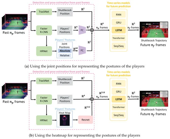
The proposed method comprises two modules: a detection and pose estimation module for past frames and a time-series model module for future prediction. Shuttlecock position, player position, and player posture information are used as input for trajectory prediction. We will be comparing fasterRCNN and tracknet and will be using the best algorithm.
What is faster R-CNN?
The Fast R-CNN detector includes a CNN backbone, an ROI pooling layer, and fully connected layers with sibling branches for classification and bounding box regression.
The input image is processed by the backbone CNN to produce a feature map (Size: 60x40x512). Using an RPN as a proposal generator enhances efficiency and leverages weight sharing between RPN and Fast R-CNN detector backbones.
RPN-generated bounding box proposals are used to extract features via the ROI pooling layer. This layer selects proposal regions, divides them into fixed sub-windows, and applies max-pooling, resulting in a (N, 7, 7, 512) output. After passing through two fully connected layers, features feed into the classification and regression branches.
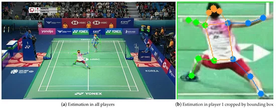
Pose estimation
What is Tracknet and why we are using this?
TrackNet is a heatmap-based deep learning network that can not only recognize the shuttle cock from a single frame but also learn flying patterns from consecutive frames, which enables the model to precisely estimate the location of the ball even when it is occluded from the players or objects.
The precision, recall, and F1-measure of TrackNet are 99.7%, 97.3%, and 98.5%, respectively, which is significantly higher than the conventional image processing method called, Archana’s algorithm
Note:
The mean diameter of a standard shuttlecock, as specified by the Badminton World Federation (BWF), is between 2.5 and 2.8 centimeters. In the context of digital representation, if we assume the mean diameter is 5 pixels, and the prediction error within a unit size of the shuttlecock does not lead to misleading trajectory identification, we can define the positioning error (PE) specification as 5 pixels. Detections with a PE greater than 5 pixels are considered false predictions.
Detection and Pose Estimation from Past Frames
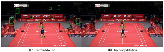
Shuttlecock position is obtained from a shuttlecock detector, while player detection and pose estimation use Faster R-CNN and HRNet, respectively. The player's position information is represented as four-dimensional coordinates, and the player's posture is captured as a 68-dimensional feature vector.
Time Series Model for Future Prediction
The combined information is fed into an LSTM network for trajectory prediction. The method is trained on a dataset, and the mean squared error is employed as the loss function.
Experiment
Dataset
The study utilizes the shuttlecock trajectory dataset, containing match videos from professional badminton tournaments. Data cleansing and augmentation are performed to enhance prediction accuracy.

The dataset is created for the model training and testing of TrackNet and TrackNetV2 for badminton applications. The dataset is composed of 26 broadcast videos. The resolution and frame rate of videos are 1280×720 and 30 fps, respectively.
A rally is a record starting from serving to its score. There are 78200 frames in total. Below are snapshots from the 23 videos. The first 23 of the video (68675 frames) is from a professional game, and the last 3 of the video (9525 frames) are playing for fun.
Model selection
A model composed of two core modules: trajectory prediction and rectification. The trajectory prediction module leverages an estimated background as auxiliary data to locate the shuttlecock in spite of the fluctuating visual interferences.
This module also incorporates mixup data augmentation to formulate complex scenarios to strengthen the network’s robustness. Given that a shuttlecock can occasionally be obstructed, we create repair masks by analyzing the predicted trajectory, subsequently rectifying the path via inpainting.
Let's start training our model
We will be using tracknet as backbone for this code however we are also considering HXnet for pose estimation.
Step 1: Prepare the dataset
Download the dataset Shuttlecock Trajectory dataset
Step 2 : Preprocessing the data
Let's preprocess the data into the required format Let's make a file named "preprocess.py" It loads the CSV in the test directory and generates the frames from the videos
import os
import parse
import shutil

from dataset import data_dir
from utils.general import list_dirs, generate_data_frames, get_num_frames, get_match_median
from utils.visualize import plot_median_files


# Replace csv to corrected csv in test set
if os.path.exists('corrected_test_label'):
    match_dirs = list_dirs(os.path.join(data_dir, 'test'))
    match_dirs = sorted(match_dirs, key=lambda s: int(s.split('match')[-1]))
    for match_dir in match_dirs:
        file_format_str = os.path.join('{}', 'test', '{}')
        _, match_dir = parse.parse(file_format_str, match_dir)
        if not os.path.exists(os.path.join(data_dir, 'test', match_dir, 'corrected_csv')):
            shutil.copytree(os.path.join('corrected_test_label', match_dir, 'corrected_csv'),
                            os.path.join(data_dir, 'test', match_dir, 'corrected_csv'))

# Generate frames from videos
for split in ['train', 'test']:
    split_frame_count = 0
    match_dirs = list_dirs(os.path.join(data_dir, split))
    for match_dir in match_dirs:
        match_frame_count = 0
        file_format_str = os.path.join('{}', 'match{}')
        _, match_id = parse.parse(file_format_str, match_dir)
        video_files = list_dirs(os.path.join(match_dir, 'video'))
        for video_file in video_files:
            generate_data_frames(video_file)
            file_format_str = os.path.join('{}', 'video', '{}.mp4')
            _, video_name = parse.parse(file_format_str, video_file)
            rally_dir = os.path.join(match_dir, 'frame', video_name)
            video_frame_count = get_num_frames(rally_dir)
            print(f'[{split} / match{match_id} / {video_name}]\tvideo frames:
            {video_frame_count}')
            match_frame_count += video_frame_count
        get_match_median(match_dir)
        print(f'[{split} / match{match_id}]:\ttotal frames: {match_frame_count}')
        split_frame_count += match_frame_count

    print(f'[{split}]:\ttotal frames: {split_frame_count}')

# Form validation set
if not os.path.exists(os.path.join(data_dir, 'val')):
    match_dirs = list_dirs(os.path.join(data_dir, 'train'))
    match_dirs = sorted(match_dirs, key=lambda s: int(s.split('match')[-1]))
    for match_dir in match_dirs:
        # Pick last rally in each match as validation set
        video_files = list_dirs(os.path.join(match_dir, 'video'))
        file_format_str = os.path.join('{}', 'train', '{}', 'video','{}.mp4')
        _, match_dir, rally_id = parse.parse(file_format_str, video_files[-1])
        os.makedirs(os.path.join(data_dir, 'val', match_dir, 'csv'), exist_ok=True)
        os.makedirs(os.path.join(data_dir, 'val', match_dir, 'video'), exist_ok=True)
        shutil.move(os.path.join(data_dir, 'train', match_dir, 'csv', f'{rally_id}_ball.csv'),
                    os.path.join(data_dir, 'val', match_dir, 'csv', f'{rally_id}_ball.csv'))
        shutil.move(os.path.join(data_dir, 'train', match_dir, 'video', f'{rally_id}.mp4'),
                    os.path.join(data_dir, 'val', match_dir, 'video', f'{rally_id}.mp4'))
        shutil.move(os.path.join(data_dir, 'train', match_dir, 'frame', rally_id),
                    os.path.join(data_dir, 'val', match_dir, 'frame', rally_id))
        shutil.copy(os.path.join(data_dir, 'train', match_dir, 'median.npz'),
                    os.path.join(data_dir, 'val', match_dir, 'median.npz'))

# Plot median frames, save at <data_dir>/median
plot_median_files(data_dir)

print('Done.')
Now we have to work on the model for this we will be using Pytorch
Step 3: Model architecture
We will be taking 7 classes for this
- Conv2DBlock
- Double2DConv
- Triple2DConv
- TrackNet
- Conv1DBlock
- Double1DConv
- InpaintNet
import torch
import torch.nn as nn

class Conv2DBlock(nn.Module):
    """ Conv2D + BN + ReLU """
    def __init__(self, in_dim, out_dim, **kwargs):
        super(Conv2DBlock, self).__init__(**kwargs)
        self.conv = nn.Conv2d(in_dim, out_dim, kernel_size=3, padding='same', bias=False)
        self.bn = nn.BatchNorm2d(out_dim)
        self.relu = nn.ReLU()

    def forward(self, x):
        x = self.conv(x)
        x = self.bn(x)
        x = self.relu(x)
        return x

class Double2DConv(nn.Module):
    """ Conv2DBlock x 2 """
    def __init__(self, in_dim, out_dim):
        super(Double2DConv, self).__init__()
        self.conv_1 = Conv2DBlock(in_dim, out_dim)
        self.conv_2 = Conv2DBlock(out_dim, out_dim)

    def forward(self, x):
        x = self.conv_1(x)
        x = self.conv_2(x)
        return x

class Triple2DConv(nn.Module):
    """ Conv2DBlock x 3 """
    def __init__(self, in_dim, out_dim):
        super(Triple2DConv, self).__init__()
        self.conv_1 = Conv2DBlock(in_dim, out_dim)
        self.conv_2 = Conv2DBlock(out_dim, out_dim)
        self.conv_3 = Conv2DBlock(out_dim, out_dim)

    def forward(self, x):
        x = self.conv_1(x)
        x = self.conv_2(x)
        x = self.conv_3(x)
        return x

class TrackNet(nn.Module):
    def __init__(self, in_dim, out_dim):
        super(TrackNet, self).__init__()
        self.down_block_1 = Double2DConv(in_dim, 64)
        self.down_block_2 = Double2DConv(64, 128)
        self.down_block_3 = Triple2DConv(128, 256)
        self.bottleneck = Triple2DConv(256, 512)
        self.up_block_1 = Triple2DConv(768, 256)
        self.up_block_2 = Double2DConv(384, 128)
        self.up_block_3 = Double2DConv(192, 64)
        self.predictor = nn.Conv2d(64, out_dim, (1, 1))
        self.sigmoid = nn.Sigmoid()

    def forward(self, x):
      x1 = self.down_block_1(x)                                       # (N,   64,  288,   512)
      x = nn.MaxPool2d((2, 2), stride=(2, 2))(x1)                     # (N,   64,  144,   256)
      x2 = self.down_block_2(x)                                       # (N,  128,  144,   256)
      x = nn.MaxPool2d((2, 2), stride=(2, 2))(x2)                     # (N,  128,   72,   128)
      x3 = self.down_block_3(x)                                       # (N,  256,   72,   128)
      x = nn.MaxPool2d((2, 2), stride=(2, 2))(x3)                     # (N,  256,   36,    64)
      x = self.bottleneck(x)                                          # (N,  512,   36,    64)
      x = torch.cat([nn.Upsample(scale_factor=2)(x), x3], dim=1)      # (N,  768,   72,   128)
      x = self.up_block_1(x)                                          # (N,  256,   72,   128)
      x = torch.cat([nn.Upsample(scale_factor=2)(x), x2], dim=1)      # (N,  384,  144,   256)
      x = self.up_block_2(x)                                          # (N,  128,  144,   256)
      x = torch.cat([nn.Upsample(scale_factor=2)(x), x1], dim=1)      # (N,  192,  288,   512)
      x = self.up_block_3(x)                                          # (N,   64,  288,   512)
      x = self.predictor(x)                                           # (N,    3,  288,   512)
      x = self.sigmoid(x)                                             # (N,    3,  288,   512)
        return x


class Conv1DBlock(nn.Module):
    """ Conv1D + LeakyReLU"""
    def __init__(self, in_dim, out_dim, **kwargs):
        super(Conv1DBlock, self).__init__(**kwargs)
        self.conv = nn.Conv1d(in_dim, out_dim, kernel_size=3, padding='same', bias=True)
        self.relu = nn.LeakyReLU()

    def forward(self, x):
        x = self.conv(x)
        x = self.relu(x)
        return x

class Double1DConv(nn.Module):
    """ Conv1DBlock x 2"""
    def __init__(self, in_dim, out_dim):
        super(Double1DConv, self).__init__()
        self.conv_1 = Conv1DBlock(in_dim, out_dim)
        self.conv_2 = Conv1DBlock(out_dim, out_dim)

    def forward(self, x):
        x = self.conv_1(x)
        x = self.conv_2(x)
        return x

class InpaintNet(nn.Module):
    def __init__(self):
        super(InpaintNet, self).__init__()
        self.down_1 = Conv1DBlock(3, 32)
        self.down_2 = Conv1DBlock(32, 64)
        self.down_3 = Conv1DBlock(64, 128)
        self.buttleneck = Double1DConv(128, 256)
        self.up_1 = Conv1DBlock(384, 128)
        self.up_2 = Conv1DBlock(192, 64)
        self.up_3 = Conv1DBlock(96, 32)
        self.predictor = nn.Conv1d(32, 2, 3, padding='same')
        self.sigmoid = nn.Sigmoid()

    def forward(self, x, m):
        x = torch.cat([x, m], dim=2)                                   # (N,   L,   3)
        x = x.permute(0, 2, 1)                                         # (N,   3,   L)
        x1 = self.down_1(x)                                            # (N,  16,   L)
        x2 = self.down_2(x1)                                           # (N,  32,   L)
        x3 = self.down_3(x2)                                           # (N,  64,   L)
        x = self.buttleneck(x3)                                        # (N,  256,  L)
        x = torch.cat([x, x3], dim=1)                                  # (N,  384,  L)
        x = self.up_1(x)                                               # (N,  128,  L)
        x = torch.cat([x, x2], dim=1)                                  # (N,  192,  L)
        x = self.up_2(x)                                               # (N,   64,  L)
        x = torch.cat([x, x1], dim=1)                                  # (N,   96,  L)
        x = self.up_3(x)                                               # (N,   32,  L)
        x = self.predictor(x)                                          # (N,   2,   L)
        x = self.sigmoid(x)                                            # (N,   2,   L)
        x = x.permute(0, 2, 1)                                         # (N,   L,   2)
        return x
Note: This is a high-level code review and It will not cover whole model processing and training guide for more details you can follow this github repository
Step 4: Model prediction
Now we have a model, we can train this model and we can also set our custom hyperparameters in the code provided above according to the use case.
Now let's get the prediction and save that prediction in a CSV file.
Network Training
Functions:
- mixup(x, y, alpha): Implements mixup, a data augmentation technique for training deep neural networks. It combines pairs of inputs and targets based on a random beta distribution.
- get_random_mask(mask_size, mask_ratio): Generates a random binary mask with a specified ratio of the masked area.
- train_tracknet(model, optimizer, data_loader, param_dict): Trains the TrackNet model for one epoch. It includes mixup, loss calculation, and visualization of predictions during training.
- train_inpaintnet(model, optimizer, data_loader, param_dict): Trains the InpaintNet model for one epoch. It involves inpainting using a random mask, loss calculation, and visualization of predictions during training.
- The script then iterates over epochs, performing training and validation steps, saving models and logging information.
- The training loop includes a learning rate scheduler, and the best model is saved based on validation accuracy.
Data Augmentation Values
Experiments are conducted with different probabilities of left–right flipping and ranges of parallel shifts to evaluate the impact of data augmentation.
The Number of Frames of Past/Future
Experiments are performed by varying the number of past and future frames to assess the model's performance.
3. Results:

4. Discussion and Conclusions
Limitation
The study acknowledges limitations in terms of camera position and adaptation to sudden changes in trajectory. Practical scenarios may require further validation of the model's generalization across different datasets and sports events.
Future Work
Future work should focus on improving the model's generalization performance and extending trajectory prediction to 3D space. Testing the model on diverse datasets and addressing sudden trajectory changes are essential for real-world applicability.
Conclusions
To sum up, TrackNet is a valid way to use computer vision to track a high-speed moving object. One of the biggest advantages of TrackNet is that it overcomes the issues of blurry and remnant images and can even detect occluded balls by learning their trajectory patterns.
To annotate these images faster you can check out Labellerr tool .
Looking for high quality training data to train your pose estimation model? Talk to our team to get a tool demo.

Simplify Your Data Annotation Workflow With Proven Strategies
.png)