Top methods to evaluate the performance of deep learning models

Even if you spend all day training supervised machine learning models, you will never be able to tell if your model is actually useful unless you test it. This in-depth talk discusses the key performance measures you need to take into account and provides clear explanations of their meaning and operation.

In this blog, you will go through the several methods for evaluating the effectiveness of our deep learning or machine learning model as well as the benefits of using one over the other. Let's first understand about deep learning.

What is deep learning?

Through the use of a machine learning approach called deep learning, computers are taught to learn by doing just like people do. Driverless cars use deep learning as a vital technology to recognize stop signs and tell a person from a lamppost apart.

Recently, deep learning has attracted a lot of interest, and for legitimate reasons. It is producing outcomes that were previously unattainable.

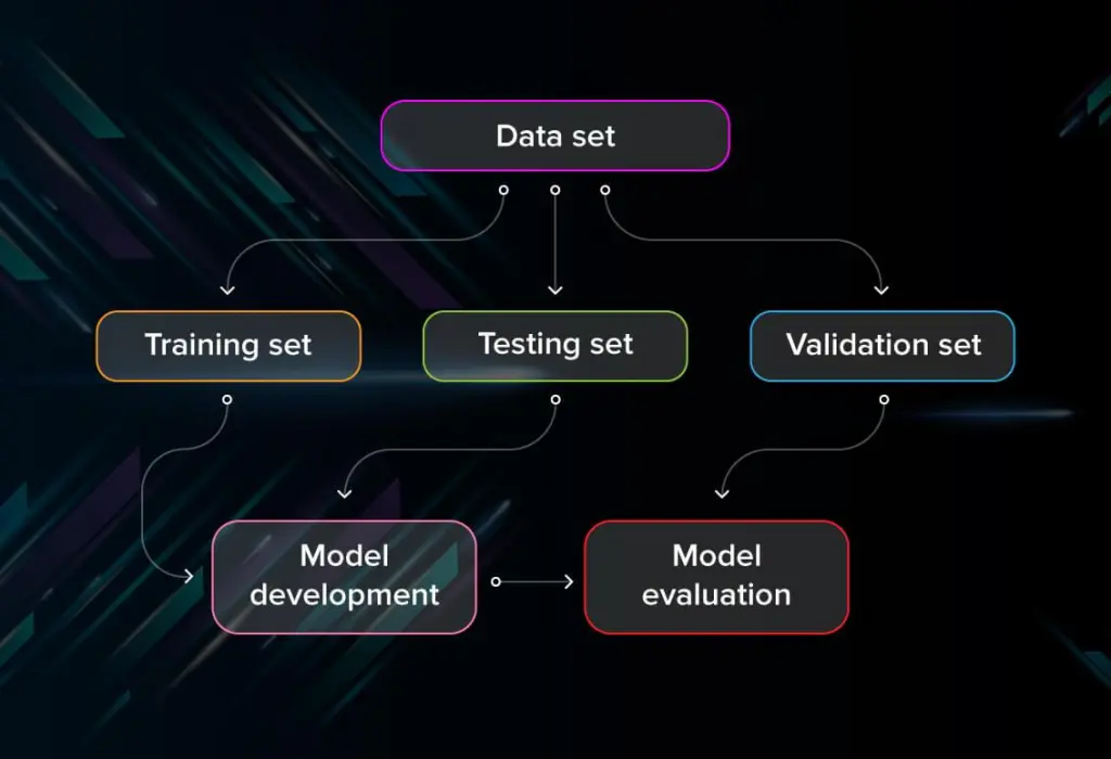
Deep learning is the process through which a computer model directly learns to carry out categorization tasks from images, texts, or sounds. Modern precision can be attained by deep learning models, sometimes even outperforming human ability. A sizable collection of labeled data and multi-layered neural network architectures are used to train models.

How does deep learning operate?

While self-learning representations are a hallmark of deep learning models, they also rely on ANNs that simulate how the brain processes information. In order to extract features, classify objects, and identify relevant data patterns, algorithms exploit independent variables in the likelihood function throughout the training phase. This takes place on several levels, employing the algorithms to create the models, much like training computers to learn for themselves.

Several algorithms are used by deep learning models. Although no network is thought to be flawless, some algorithms are more effective at carrying out particular tasks. It's beneficial to develop a thorough understanding of all major algorithms in order to make the best choices.

Methods to evaluate the performance of a deep learning model-

1. Confusion Matrix

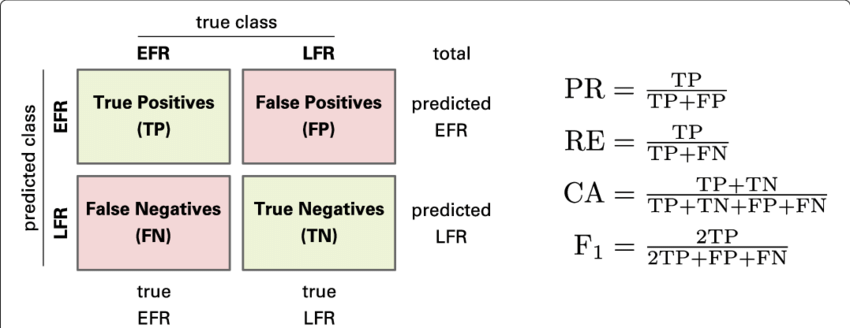
Confusion Matrix to assess model effectiveness Parameters are displayed as a matrix using a confusion matrix. It enables us to see real and fake positives as well as fake negatives. We can divide the total number of tests by the total number of false positives and false negatives to obtain the overall accuracy. A confusion matrix can be used by importing it via the Sklearn library. Python's Scikit-learn (sklearn) offers tools for statistical modelling and machine learning, ranging from classification via methods for dimensionality reduction.

2. Accuracy

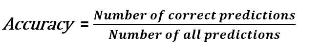
The most popular metric for evaluating a model isn't a good predictor of how well it will perform. When classrooms are unbalanced, the worst happens. As its name implies, accuracy is a measurement of how accurate a model is.

Accuracy = Correct Predictions / Total Predictions

By using confusion matrix, Accuracy = (TP + TN)/(TP+TN+FP+FN)

Consider a model for detecting cancer. Cancer is extremely unlikely to actually exist. If there are 100 patients, let's assume 90 of them are cancer-free, and the other 10 are. We don't want to overlook a patient with cancer who remains undiagnosed (false negative). 90% of the time, everyone is correctly identified as cancer-free. Here, the model did little but provide a cancer-free outcome for each of the 100 forecasts.

3. Precision

Precision is the proportion of true positives to all expected true positives. The denominator is the total number of positives created, true or false, and the numerator is the total number of true positives. The numerator of the equation below only includes genuine positives, whereas the denominator includes both true and false positives. This equation tells us how frequently

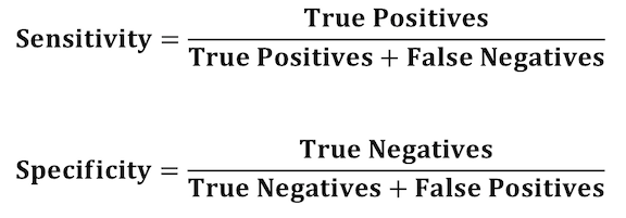
4. Recall or true positive rate

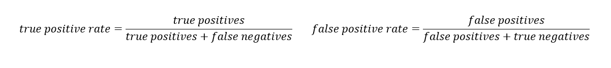
True Positive Rate or Recall Recall captures the proportion of positive instances among all actual positive cases. The "positive examples" in this instance are values produced by the model, however the "total true positive instances" are supported by test data. The number of real positive cases in the collection will therefore serve as the denominator (false negatives, true positives). We use the proportion of positives known based on verified data rather than the overall number of positives created by the model as was done for the deep learning precision (above). This equation reveals how many more positives the model reported when it should have been negative.

5. PR Curve

It represents the curve between recall and precision for different threshold settings. Six predictors are represented in the figure below, each with a precision-recall curve for a range of threshold values. The optimal location for excellent precision and recall is in the top right corner of the graph. We can select the threshold value and the predictor based on our application. Simply said, PR AUC is the region under the curve. The better, the greater the numerical value.

In situations where classes are not fairly distributed, precision and recall are helpful. The typical example is creating a classification system that can determine if a person has a sickness or not. We might create a classifier that consistently predicts that a person doesn't even have the disease if only a small portion of the population (let's assume 1%), in which case our model would be 99% correct but 0% useful.

However, it would be obvious that our model was flawed if we examined the recall of this pointless prediction. In this case, recall makes sure we don't miss the disease-carriers, while accuracy guards against incorrectly labeling too many individuals as carriers when they aren't. Naturally, you don't want a model which forecasts someone has cancer when they actually do not, but you also wouldn't want one that predicts others do not have cancer when they actually do. Therefore, it's crucial to assess a model's precision and recall.

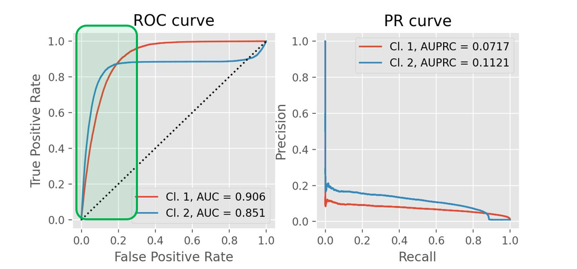
6. ROC graph

Receiver operating characteristic, or ROC,can be seen on a graph together with TPR and FPR at various threshold levels. TPR and FPR both rise when TPR does. We have four categories, as shown in the first picture, and our goal is to go as close to the top left corner as possible by the threshold value. Choosing the threshold involves the application at hand making comparing various classifiers (here 3) on a particular dataset simple. The better the ROC AUC's numerical value, which is just the regression coefficient.

7. Specificity of a Model

Deep learning Models' Specificity: the fraction of negative cases relative to all genuine negative instances is what is meant by specificity. It is comparable to the previous true positive rate approach. In this case, the denominator represents the total of real values that were validated by data rather than being produced by the model. This formula allows us to evaluate how well the model is appropriate when it creates negative outputs depending on the negatives of the overall negatives it created in the past because the numerator denotes the amount of true negatives.

8. F1 Score

F1 Score for Deep Learning Model Analysis The F1 score is calculated by averaging precision and recall. Since both of them must be included, the more precise the model, the greater the F1 score. On the other hand, if the numerator's product falls too far, the F1 score plummets sharply. The greatest extreme ratios of "true:false" positives and "true:false" negatives are found in models with high F1 scores. An effective F1 score, for instance, will be produced if the ratio of genuine positives to false positives is 100:1. A low F1 score will result from a close ratio of true to false - positive, such as 50:51.

Conclusion

In summary, you should thoroughly understand the data set and problem before creating a confusion matrix and testing its accuracy, precision, and recall. You can then display the ROC curve and get the AUC according to your needs. However, you should never use precision as a metric if your data collection is unbalanced. Consider using Log Loss if you want to further analyze your model and assign weight to your probability values. Never forget to assess your training!

Find this blog helpful, want to read more-Check out our blog section!