A Comprehensive Guide To Build Farm Insect Detection Model

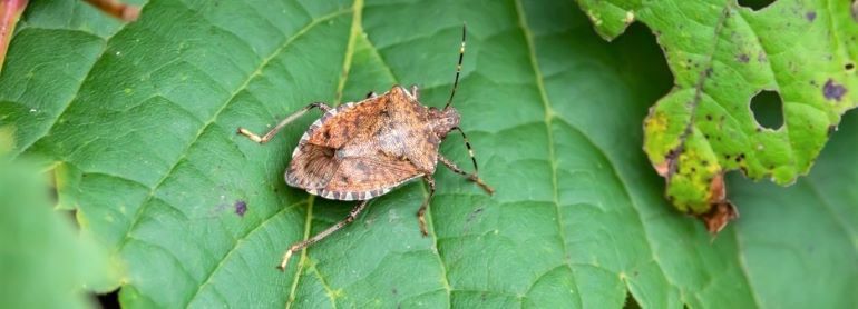
Table of Contents

1. Introduction
2. Data Collection and Preprocessing
3. Model Configuration and Training
4. Analysis and Visualization
5. Inference and Deployment
6. Conclusion
7. Future Considerations
8. Frequently Asked Questions

Introduction

Deep learning and other cutting-edge technologies are now helping the agriculture industry, which is essential for the world's sustenance. Using a bespoke dataset and a pre-trained model, we investigate the use of Vision Transformers (ViT) for farm insect detection in this blog. We'll go over the essential procedures for putting into practice a reliable system for recognizing harmful insects on farms, from data preprocessing to model training and assessment.

LabelGPT: Auto Detect Object In Multiple Datasets

Get Automatic Prediction In Just One Click

1.Data Collection and Preprocessing

The first step involves collecting and organizing the dataset. In this case, images of dangerous insects on farms are gathered, and their corresponding labels are extracted from file paths.

# Importing necessary libraries and modules
import warnings  # Import the 'warnings' module for handling warnings
warnings.filterwarnings("ignore")  # Ignore warnings during execution

import gc  # Import the 'gc' module for garbage collection
import numpy as np  # Import NumPy for numerical operations
import pandas as pd  # Import Pandas for data manipulation
import itertools  # Import 'itertools' for iterators and looping
from collections import Counter  # Import 'Counter' for counting elements
import matplotlib.pyplot as plt  # Import Matplotlib for data visualization
from sklearn.metrics import (  # Import various metrics from scikit-learn
    accuracy_score,  # For calculating accuracy
    roc_auc_score,  # For ROC AUC score
    confusion_matrix,  # For confusion matrix
    classification_report,  # For classification report
    f1_score  # For F1 score
)

# Import custom modules and classes
from imblearn.over_sampling import RandomOverSampler # import RandomOverSampler
import evaluate  # Import the 'evaluate' module
from datasets import Dataset, Image, ClassLabel  # Import custom 'Dataset', 
'ClassLabel', and 'Image' classes
from transformers import (  # Import various modules from the Transformers library
    TrainingArguments,  # For training arguments
    Trainer,  # For model training
    ViTImageProcessor,  # For processing image data with ViT models
    ViTForImageClassification,  # ViT model for image classification
    DefaultDataCollator  # For collating data in the default way
)
import torch  # Import PyTorch for deep learning
from torch.utils.data import DataLoader  # For creating data loaders
from torchvision.transforms import (  # Import image transformation functions
    CenterCrop,  # Center crop an image
    Compose,  # Compose multiple image transformations
    Normalize,  # Normalize image pixel values
    RandomRotation,  # Apply random rotation to images
    RandomResizedCrop,  # Crop and resize images randomly
    RandomHorizontalFlip,  # Apply random horizontal flip
    RandomAdjustSharpness,  # Adjust sharpness randomly
    Resize,  # Resize images
    ToTensor  # Convert images to PyTorch tensors
)

# Import the necessary module from the Python Imaging Library (PIL).
from PIL import ImageFile

# Enable the option to load truncated images.
# This setting allows the PIL library to attempt loading images even if they are 
corrupted or incomplete.
ImageFile.LOAD_TRUNCATED_IMAGES = True

# Import necessary libraries
image_dict = {}

# Define the list of file names
from pathlib import Path
from tqdm import tqdm
import os
# Initialize empty lists to store file names and labels
file_names = []
labels = []

# Iterate through all image files in the specified directory
for file in tqdm(sorted((Path('/kaggle/input/dangerous-insects-
dataset/farm_insects/').glob('*/*.*')))):
    label = str(file).split('/')[-2]  # Extract the label from the file path
    labels.append(label)  # Add the label to the list
    file_names.append(str(file))  # Add the file path to the list

# Print the total number of file names and labels
print(len(file_names), len(labels))

# Create a pandas dataframe from the collected file names and labels
df = pd.DataFrame.from_dict({"image": file_names, "label": labels})
print(df.shape)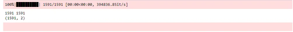

df.head()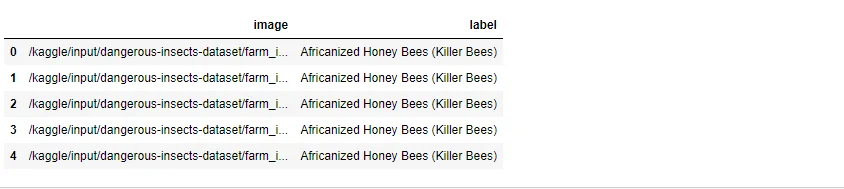

df['label'].unique()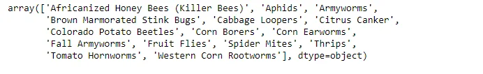

To address class imbalance, random oversampling of the minority class is performed using the RandomOverSampler from the imbalanced-learn library.

# random oversampling of minority class
# 'y' contains the target variable (label) we want to predict
y = df[['label']]

# Drop the 'label' column from the DataFrame 'df' to separate features from the target variable
df = df.drop(['label'], axis=1)

# Create a RandomOverSampler object with a specified random seed (random_state=83)
ros = RandomOverSampler(random_state=83)

# Use the RandomOverSampler to resample the dataset by oversampling the minority class
# 'df' contains the feature data, and 'y_resampled' will contain the resampled target variable
df, y_resampled = ros.fit_resample(df, y)

# Delete the original 'y' variable to save memory as it's no longer needed
del y

# Add the resampled target variable 'y_resampled' as a new 'label' column in the DataFrame 'df'
df['label'] = y_resampled

# Delete the 'y_resampled' variable to save memory as it's no longer needed
del y_resampled

# Perform garbage collection to free up memory used by discarded variables
gc.collect()

print(df.shape)

The dataset is converted into a custom format compatible with deep learning frameworks, utilizing the Dataset class. Each image is associated with a specific label, creating a structured input for the model.

# Create a dataset from a Pandas DataFrame.
dataset = Dataset.from_pandas(df).cast_column("image", Image())

# Display the first image in the dataset
dataset[0]["image"]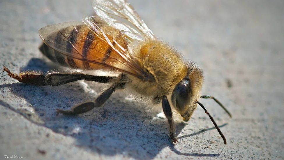

labels_subset = labels[:5]

# Printing the subset of labels to inspect the content.
print(labels_subset)

# Create a list of unique labels by converting 'labels' to a set and then back to a list
labels_list = list(set(labels))

# Initialize empty dictionaries to map labels to IDs and vice versa
label2id, id2label = dict(), dict()

# Iterate over the unique labels and assign each label an ID, and vice versa
for i, label in enumerate(labels_list):
    label2id[label] = i  # Map the label to its corresponding ID
    id2label[i] = label  # Map the ID to its corresponding label

# Print the resulting dictionaries for reference
print("Mapping of IDs to Labels:", id2label, '\n')
print("Mapping of Labels to IDs:", label2id)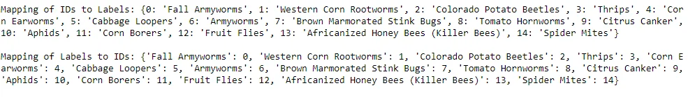

# Creating classlabels to match labels to IDs
ClassLabels = ClassLabel(num_classes=len(labels_list), names=labels_list)

# Mapping labels to IDs
def map_label2id(example):
    example['label'] = ClassLabels.str2int(example['label'])
    return example

dataset = dataset.map(map_label2id, batched=True)

# Casting label column to ClassLabel Object
dataset = dataset.cast_column('label', ClassLabels)

# Splitting the dataset into training and testing sets using an 80-20 split ratio.
dataset = dataset.train_test_split(test_size=0.2, shuffle=True, stratify_by_column="label")

# Extracting the training data from the split dataset.
train_data = dataset['train']

# Extracting the testing data from the split dataset.
test_data = dataset['test']

2.Model Configuration and Training

A pre-trained Vision Transformer (ViT) model is chosen for its effectiveness in image classification tasks. The selected model is configured with the appropriate number of output labels.

# Define the pre-trained ViT model string
model_str = 'google/vit-base-patch16-224-in21k'

# Create a processor for ViT model input from the pre-trained model
processor = ViTImageProcessor.from_pretrained(model_str)

# Retrieve the image mean and standard deviation used for normalization
image_mean, image_std = processor.image_mean, processor.image_std

# Get the size (height) of the ViT model's input images
size = processor.size["height"]
print("Size: ", size)

# Define a normalization transformation for the input images
normalize = Normalize(mean=image_mean, std=image_std)

# Define a set of transformations for training data
_train_transforms = Compose(
    [
        Resize((size, size)),             # Resize images to the ViT model's input size
        RandomRotation(90),               # Apply random rotation
        RandomAdjustSharpness(2),         # Adjust sharpness randomly
        ToTensor(),                       # Convert images to tensors
        normalize                         # Normalize images using mean and std
    ]
)

# Define a set of transformations for validation data
_val_transforms = Compose(
    [
        Resize((size, size)),             # Resize images to the ViT model's input size
        ToTensor(),                       # Convert images to tensors
        normalize                         # Normalize images using mean and std
    ]
)

# Define a function to apply training transformations to a batch of examples
def train_transforms(examples):
    examples['pixel_values'] = [_train_transforms(image.convert("RGB")) for image
    in examples['image']]
    return examples

# Define a function to apply validation transformations to a batch of examples
def val_transforms(examples):
    examples['pixel_values'] = [_val_transforms(image.convert("RGB")) for image in
    examples['image']]
    return examples

# Set the transforms for the training data
train_data.set_transform(train_transforms)

# Set the transforms for the test/validation data
test_data.set_transform(val_transforms)	

# Define a collate function that prepares batched data for model training.
def collate_fn(examples):
    # Stack the pixel values from individual examples into a single tensor.
    pixel_values = torch.stack([example["pixel_values"] for example in examples])
    
    # Convert the label strings in examples to corresponding numeric IDs using 
    label2id dictionary.
    labels = torch.tensor([example['label'] for example in examples])
    
    # Return a dictionary containing the batched pixel values and labels.
    return {"pixel_values": pixel_values, "labels": labels}

Training is configured using the TrainingArguments class, specifying parameters such as learning rate, batch size, and the number of training epochs. The model is fine-tuned on the prepared dataset.

# Create a ViTForImageClassification model from a pretrained checkpoint with a 
specified number of output labels.
model = ViTForImageClassification.from_pretrained(model_str, num_labels=len(labels_list))

# Configure the mapping of class labels to their corresponding indices for later reference.
model.config.id2label = id2label
model.config.label2id = label2id

# Calculate and print the number of trainable parameters in millions for the model.
print(model.num_parameters(only_trainable=True) / 1e6)

# Load the accuracy metric from a module named 'evaluate'
accuracy = evaluate.load("accuracy")

# Define a function 'compute_metrics' to calculate evaluation metrics
def compute_metrics(eval_pred):
    # Extract model predictions from the evaluation prediction object
    predictions = eval_pred.predictions
    
    # Extract true labels from the evaluation prediction object
    label_ids = eval_pred.label_ids
    
    # Calculate accuracy using the loaded accuracy metric
    # Convert model predictions to class labels by selecting the class with the
    highest probability (argmax)
    predicted_labels = predictions.argmax(axis=1)
    
    # Calculate accuracy score by comparing predicted labels to true labels
    acc_score = accuracy.compute(predictions=predicted_labels, 
    references=label_ids)['accuracy']
    
    # Return the computed accuracy as a dictionary with the key "accuracy"
    return {
        "accuracy": acc_score
    }

# Define the name of the evaluation metric to be used during training and evaluation.
metric_name = "accuracy"

# Define the name of the model, which will be used to create a directory for
saving model checkpoints and outputs.
model_name = "farm_insects_image_detection"

# Define the number of training epochs for the model.
num_train_epochs = 40

# Create an instance of TrainingArguments to configure training settings.
args = TrainingArguments(
    # Specify the directory where model checkpoints and outputs will be saved.
    output_dir=model_name,
    
    # Specify the directory where training logs will be stored.
    logging_dir='./logs',
    
    # Define the evaluation strategy, which is performed at the end of each epoch.
    evaluation_strategy="epoch",
    
    # Set the learning rate for the optimizer.
    learning_rate=1e-5,
    
    # Define the batch size for training on each device.
    per_device_train_batch_size=64,
    
    # Define the batch size for evaluation on each device.
    per_device_eval_batch_size=32,
    
    # Specify the total number of training epochs.
    num_train_epochs=num_train_epochs,
    
    # Apply weight decay to prevent overfitting.
    weight_decay=0.02,
    
    # Set the number of warm-up steps for the learning rate scheduler.
    warmup_steps=50,
    
    # Disable the removal of unused columns from the dataset.
    remove_unused_columns=False,
    
    # Define the strategy for saving model checkpoints (per epoch in this case).
    save_strategy='epoch',
    
    # Load the best model at the end of training.
    load_best_model_at_end=True,
    
    # Limit the total number of saved checkpoints to save space.
    save_total_limit=1,
    
    # Specify that training progress should be reported to MLflow.
    report_to="mlflow"  # log to mlflow
)

# Create a Trainer instance for fine-tuning a language model.

trainer = Trainer(
    model,
    args,
    train_dataset=train_data,
    eval_dataset=test_data,
    data_collator=collate_fn,
    compute_metrics=compute_metrics,
    tokenizer=processor,
)

The model's performance is evaluated on a test dataset, calculating metrics like accuracy and loss. Evaluation metrics provide insights into how well the model generalizes to unseen data.

# Evaluate the pre-training model's performance on a test dataset.
trainer.evaluate()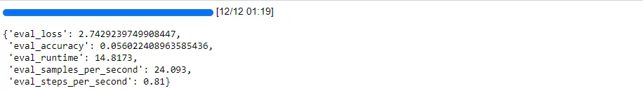

# Start training the model using the trainer object.
trainer.train()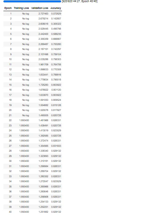

# Evaluate the post-training model's performance on the validation or test dataset.
trainer.evaluate()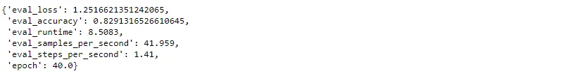

# Use the trained 'trainer' to make predictions on the 'test_data'.
outputs = trainer.predict(test_data)

# Print the metrics obtained from the prediction outputs.
print(outputs.metrics)

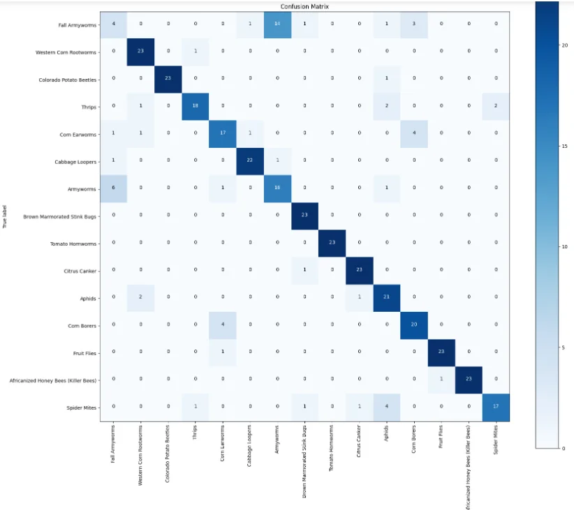
3.Analysis and Visualization

A confusion matrix is generated to visualize the model's predictions and identify areas of misclassification. This aids in understanding the model's strengths and areas for improvement.

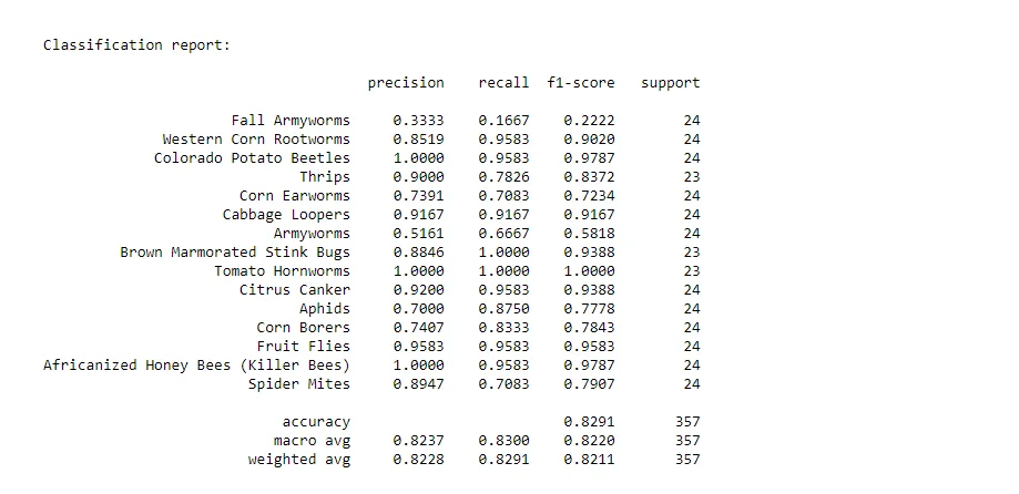
A detailed classification report is presented, including metrics such as precision, recall, and F1 score for each class. This provides a comprehensive overview of the model's performance on individual classes.

# Extract the true labels from the model outputs
y_true = outputs.label_ids

# Predict the labels by selecting the class with the highest probability
y_pred = outputs.predictions.argmax(1)

# Define a function to plot a confusion matrix
def plot_confusion_matrix(cm, classes, title='Confusion Matrix', 
cmap=plt.cm.Blues, figsize=(10, 8)):

    # Create a figure with a specified size
    plt.figure(figsize=figsize)
    
    # Display the confusion matrix as an image with a colormap
    plt.imshow(cm, interpolation='nearest', cmap=cmap)
    plt.title(title)
    plt.colorbar()

    # Define tick marks and labels for the classes on the axes
    tick_marks = np.arange(len(classes))
    plt.xticks(tick_marks, classes, rotation=90)
    plt.yticks(tick_marks, classes)

    fmt = '.0f'
    # Add text annotations to the plot indicating the values in the cells
    thresh = cm.max() / 2.0
    for i, j in itertools.product(range(cm.shape[0]), range(cm.shape[1])):
        plt.text(j, i, format(cm[i, j], fmt), horizontalalignment="center",
        color="white" if cm[i, j] > thresh else "black")

    # Label the axes
    plt.ylabel('True label')
    plt.xlabel('Predicted label')

    # Ensure the plot layout is tight
    plt.tight_layout()
    # Display the plot
    plt.show()

# Calculate accuracy and F1 score
accuracy = accuracy_score(y_true, y_pred)
f1 = f1_score(y_true, y_pred, average='macro')

# Display accuracy and F1 score
print(f"Accuracy: {accuracy:.4f}")
print(f"F1 Score: {f1:.4f}")

# Get the confusion matrix if there are a small number of labels
if len(labels_list) <= 150:
    # Compute the confusion matrix
    cm = confusion_matrix(y_true, y_pred)

    # Plot the confusion matrix using the defined function
    plot_confusion_matrix(cm, labels_list, figsize=(18, 16))
    
# Finally, display classification report
print()
print("Classification report:")
print()
print(classification_report(y_true, y_pred, target_names=labels_list, digits=4))

4.Inference and Deployment

The trained model is saved for future use, ensuring that the fine-tuned weights and configurations are preserved.

trainer.save_model()

A pipeline for making predictions on new images is established using the transformers library. This enables seamless deployment of the model for real-time inference.

from transformers import pipeline

pipe = pipeline('image-classification', model=model_name, device=0)

image = test_data[1]["image"]

image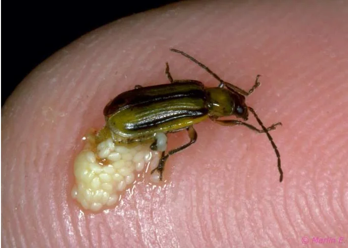

# Apply the 'pipe' function to process the 'image' variable.
pipe(image)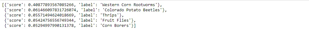

# This line of code accesses the "label" attribute of a specific element in the test_data list.
# It's used to retrieve the actual label associated with a test data point.
id2label[test_data[1]["label"]]

Conclusion

The blog concludes by highlighting the real-world uses for deep learning-based farm insect identification. Precision agricultural techniques benefit from the model's capacity to recognise harmful insects since it allows for prompt responses and less crop damage.

Future Considerations

1.Model Fine-Tuning

The model can be improved to perform better on particular bug species or environmental conditions as additional data become available.

2.Integration with Farming Systems

Exploring the possibilities of integrating the insect detection model for real-time monitoring and decision-making with the farming equipment and systems now in use.

3.Community Engagement

Emphasising the significance of community involvement in data gathering, model verification, and tackling regional obstacles associated with agricultural insect identification.

This blog seeks to provide agricultural stakeholders with the information and resources necessary to apply deep learning solutions for farm pest detection, resulting in a more resilient and sustainable agricultural ecosystem.

Frequently Asked Questions

1.What is machine vision how can it be attained by using deep learning?

Voice recognition and machine vision are comparable in complexity. The terms "computer vision" and "machine vision" are sometimes used interchangeably. To speed up image processing, the technology is frequently combined with deep learning, machine learning, and artificial intelligence (AI).

2.How deep learning helps in agriculture?

When combined with machine-learning (ML) methods, deep learning (DL) can assist farmers in comprehending the characteristics of their soil, which will help them make informed farming decisions on time. DL is also used to determine the best time to plant and harvest crops, as well as to evaluate how water and nutrients should be handled.

3.What is the vision of smart agriculture?

Smart agriculture reduces greenhouse gas emissions, builds resilience to climate change, and encourages a sustainable growth in agricultural productivity and income.

4.How computer vision is used in smart agriculture?

Crop health monitoring is one of the main uses of computer vision in the agriculture sector. It uses cameras to record different stages of crop growth and boost productivity. Farmers are better able to spot minor irregularities in crop development that are first brought on by starvation.