
DINOv3 Explained: The Future of Self-Supervised Learning
DINOv3 is Meta’s open-source vision backbone trained on over a billion images using self-supervised learning. It provides pretrained models, adapters, training code, and deployment support for advanced, annotation-free vision solutions.

Imagine you need to build a system that can identify defective parts on a fast-moving assembly line. The catch? You have thousands of images of good parts, but only a handful of examples for each type of defect. Training a traditional deep learning model would be a nightmare, requiring you to manually label countless images of scratches, dents, and misalignments.
What if you could build a highly accurate system using just the images of good parts? What if a single AI model could learn what "normal" looks like so well that it could spot any deviation, even ones it has never seen before?
This isn't a hypothetical scenario. This is a challenge you can solve today with DINOv3, a groundbreaking computer vision model from Meta AI.
What is DINOv3?
DINOv3 is a powerful, general-purpose vision model that learns about the visual world through self-supervised learning. Unlike traditional models that require massive, human-labeled datasets, DINOv3 teaches itself by analyzing the relationships between different parts of an image. It learns concepts like shape, texture, and spatial relationships on its own.
Because it doesn't need labels, Meta was able to train DINOv3 on an enormous dataset of 1.7 billion images. This gives the model an incredibly rich and robust understanding of the world, making it a "foundation model" for vision—a single, powerful base that you can adapt to many different tasks.
What Are DINOv3's Key Features?
DINOv3 isn't just bigger; it's smarter. It introduces several key features that make it so effective:
- Frozen Backbone Approach: This is the model's superpower. The core model's knowledge is "frozen," meaning you don't need to retrain or fine-tune it for new tasks. This saves an enormous amount of time and computational cost.
- High-Quality Features: DINOv3 produces high-dimensional "feature vectors" that capture the essence of an image. These features are so good that even simple classifiers (like k-Nearest Neighbors) built on top of them can achieve state-of-the-art results.
- Dense and Global Understanding: The model provides both a single "global" feature vector for the entire image and a grid of "patch" features that capture details about specific regions. This makes it powerful for both classification (what's in the image?) and segmentation (where is it?).
- Open and Commercially Available: Meta has released DINOv3 with a license that allows for commercial use, opening the door for businesses to build innovative applications.
What Model Types Are Available?
DINOv3 is not a one-size-fits-all model. It comes in a family of sizes, allowing you to choose the right balance of performance and efficiency for your needs.
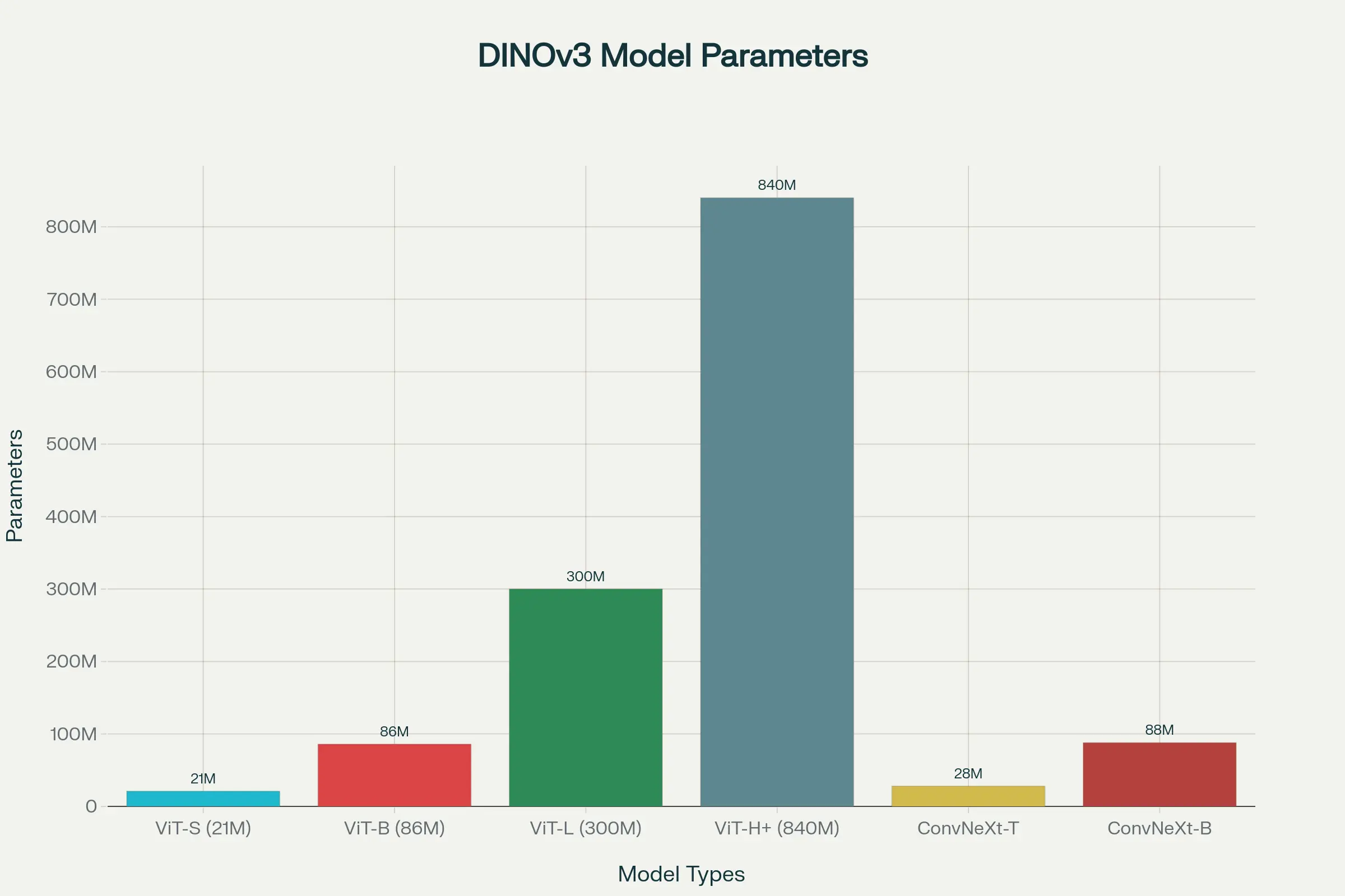
DINOv3 Model Types: Parameters and Typical Use Cases
- Vision Transformer (ViT) Models: These offer the highest performance and come in sizes from the nimble ViT-S (21M parameters) to the powerhouse ViT-H+ (840M parameters).
- ConvNeXt Models: These are designed for efficiency and are a great choice for on-device or edge computing applications where speed is critical.
What Tasks Can DINOv3 Perform?
Because DINOv3's features are so robust, you can use them for a wide array of computer vision tasks without any fine-tuning.
First we will install the required libraries.
pip install transformers torch torchvision scikit-learn matplotlib einops accelerate timm
Let's load the model and define the feature extraction helper functions:
import torch
from transformers import AutoImageProcessor, AutoModel
from transformers.image_utils import load_image
import numpy as np
# Use a smaller DINOv3 model for faster demos
model_name = "facebook/dino-vits16"
# Load the processor and model
processor = AutoImageProcessor.from_pretrained(model_name)
model = AutoModel.from_pretrained(model_name)
model.eval() # Set the model to evaluation mode

def extract_pooled_features(images):
    """Extracts the global (class token) features for a batch of images."""
    inputs = processor(images=images, return_tensors="pt")
    with torch.no_grad():
        outputs = model(**inputs)
    return outputs.pooler_output.cpu().numpy()

def extract_patch_features(image):
    """Extracts the dense patch features for a single image."""
    inputs = processor(images=image, return_tensors="pt")
    with torch.no_grad():
        outputs = model(**inputs)
    # The first token is the class token, so we skip it
    patch_features = outputs.last_hidden_state[:, 1:, :].squeeze(0).cpu().numpy()
    return patch_features

# Load some sample images from public URLs
image_urls = [
    "http://images.cocodataset.org/val2017/000000039769.jpg",  # Cat image
    "https://images.unsplash.com/photo-1583337130417-2346a1e724c2", # Dog image
    "http://images.cocodataset.org/val2017/000000004134.jpg" # Bird image
]
images = [load_image(url) for url in image_urls]
Here are just a few examples:
- Image Classification: Build highly accurate classifiers with just a few labeled examples by training a simple k-NN or logistic regression model on DINOv3's features.
from sklearn.linear_model import LogisticRegression
print("\n--- 2. Linear Classification (Combined Features) ---")

def extract_combined_features(images):
    """Extracts combined global and average patch features."""
    inputs = processor(images=images, return_tensors="pt")
    with torch.no_grad():
        outputs = model(**inputs)

    global_features = outputs.pooler_output
    patch_features = outputs.last_hidden_state[:, 1:, :].mean(dim=1)
    combined = torch.cat([global_features, patch_features], dim=1)
    return combined.cpu().numpy()

# Extract combined features
combined_features = extract_combined_features(images)

# Train a logistic regression classifier
log_reg = LogisticRegression(max_iter=1000)
log_reg.fit(combined_features, labels)

# Predict with the combined features of the dog image
test_combined_features = extract_combined_features([test_image])
prediction = log_reg.predict(test_combined_features)

print(f"Linear classifier prediction for the dog image: Class {prediction[0]}")
- Image Retrieval and Similarity Search: Create a visual search engine by comparing the feature vectors of images. Find duplicate images or products that look similar.
from sklearn.metrics.pairwise import cosine_similarity
print("\n--- 3. Image Retrieval and Similarity Search ---")

# Use the cat image as the query
query_image = images[0]
query_features = extract_pooled_features([query_image])

# Calculate cosine similarity between the query and all images
similarities = cosine_similarity(query_features, features).flatten()

# Sort images by similarity
sorted_indices = np.argsort(similarities)[::-1]

print("Image indices sorted by similarity to the cat image:", sorted_indices)
print("Similarity scores:", similarities[sorted_indices])
- Depth Estimation: The model's features contain strong geometric information, allowing you to train a simple "head" to estimate the relative depth of objects in a scene.
import torch.nn as nn
print("\n--- 4. Depth Estimation (with a simple head) ---")

class DepthHead(nn.Module):
    def __init__(self, input_dim=384): # For ViT-S/16 model
        super().__init__()
        self.head = nn.Linear(input_dim, 1)
    def forward(self, x):
        return self.head(x)

# Create a dummy depth estimation head
depth_estimator = DepthHead()
depth_estimator.eval()

# "Estimate" depth for each image
with torch.no_grad():
    depth_predictions = depth_estimator(torch.from_numpy(features))

print("Estimated relative depth values:", depth_predictions.numpy().flatten())
- Semantic Segmentation: Use the dense patch features to classify every region of an image, creating detailed segmentation maps.
print("\n--- 5. Semantic Segmentation (with a simple head) ---")

class SegmentationHead(nn.Module):
    def __init__(self, input_dim=384, num_classes=10):
        super().__init__()
        self.head = nn.Linear(input_dim, num_classes)
    def forward(self, x):
        return self.head(x)

# Create a dummy segmentation head
seg_head = SegmentationHead()
seg_head.eval()

# Get patch features for the cat image
patch_features = extract_patch_features(images[0])

# Get segmentation map
with torch.no_grad():
    segmentation_logits = seg_head(torch.from_numpy(patch_features))
    segmentation_map = torch.argmax(segmentation_logits, dim=-1)

print("Shape of the segmentation map:", segmentation_map.shape)
- 3D Keypoint Correspondences: Find matching points between two images of the same object, a critical task for 3D reconstruction.
print("\n--- 6. 3D Keypoint Correspondences ---")

# Use two different images for matching
image1 = images[0]
image2 = load_image("http://images.cocodataset.org/val2017/000000483108.jpg") # Another cat

# Get patch features
features1 = torch.from_numpy(extract_patch_features(image1))
features2 = torch.from_numpy(extract_patch_features(image2))

# Normalize features
features1 = features1 / features1.norm(dim=-1, keepdim=True)
features2 = features2 / features2.norm(dim=-1, keepdim=True)

# Find mutual nearest neighbors
similarity_matrix = torch.matmul(features1, features2.T)
nn1 = torch.argmax(similarity_matrix, dim=1)
nn2 = torch.argmax(similarity_matrix, dim=0)

mutual_matches = []
for i in range(len(nn1)):
    if nn2[nn1[i]] == i:
        mutual_matches.append((i, nn1[i].item()))

print(f"Found {len(mutual_matches)} mutual keypoint matches between the two cat images.")
- Unsupervised Object Discovery: Cluster the patch features to automatically find and segment objects in an image without any supervision.
from sklearn.cluster import KMeans
import matplotlib.pyplot as plt
print("\n--- 7. Unsupervised Object Discovery ---")

# Get patch features for the cat image
patch_features = extract_patch_features(images[0])

# Cluster the patch features
kmeans = KMeans(n_clusters=3, random_state=0, n_init=10)
clusters = kmeans.fit_predict(patch_features)

# Reshape to a 14x14 grid to visualize the clusters
cluster_map = clusters.reshape(14, 14)
plt.imshow(cluster_map, cmap='viridis')
plt.title("Unsupervised Object Clusters")
plt.show()
- Video Analysis: By processing frames individually, you can extend these capabilities to video, enabling tasks like object tracking and video classification.
print("\n--- 8. Video Segmentation Tracking ---")
# Create a dummy video (3 frames of the same cat image)
video_frames = [images[0]] * 3
frame_features = [torch.from_numpy(extract_patch_features(f)) for f in video_frames]

# Track by finding the best match for each patch in the next frame
tracked_patches = []
for i in range(len(frame_features) - 1):
    similarity = torch.matmul(frame_features[i], frame_features[i+1].T)
    best_matches = torch.argmax(similarity, dim=1)
    tracked_patches.append(best_matches)
print("Tracked patch indices between frame 0 and 1:", tracked_patches[0].tolist())

print("\n--- 9. Video Classification ---")
# A simple approach is to average the features of all frames
video_features_pooled = extract_pooled_features(video_frames)
average_video_feature = np.mean(video_features_pooled, axis=0)

# Use this average feature with a classifier like k-NN or Logistic Regression
# prediction = knn.predict([average_video_feature])
print("Shape of the average video feature vector:", average_video_feature.shape)
What's Next? Combining DINOv3 with Other Models
DINOv3 is incredibly powerful on its own, but its true potential is unlocked when you combine it with other AI models. Its rich visual features provide the perfect foundation for more complex, multimodal systems.
In our upcoming blogs, we will explore how to build these advanced systems:
- DINOv3 + CLIP: For powerful zero-shot classification and image-text retrieval.
- DINOv3 + Large Language Models (LLMs): To create systems that can "reason" about images and answer complex questions.
- DINOv3 + Vision-Language Models (VLMs): For generating detailed image captions and reports.
- DINOv3 + SAM (Segment Anything Model): For creating highly accurate, semantically-aware image segmentation.
Conclusion
DINOv3 marks a significant step forward for computer vision. It makes state-of-the-art performance accessible, affordable, and easy to deploy. By providing a powerful and versatile foundation, it allows developers and businesses to move beyond the constraints of labeled data and build the next generation of intelligent vision applications.
Whether you're building a visual search engine, an automated quality control system, or a medical imaging diagnostic tool, DINOv3 provides the features you need to solve real-world challenges quickly and effectively. The era of universal vision models is here, and DINOv3 is leading the charge.
FAQs
Q1: What is DINOv3?
DINOv3 is Meta’s open-source, self-supervised computer vision model, excelling in dense prediction and versatile visual understanding tasks.
Q2: What makes DINOv3 different from previous vision models?
Unlike older models, DINOv3 requires no image labels, delivers strong visual features across domains, and performs exceptionally without fine-tuning, enabling faster and broader adoption.
Q3: Can I deploy DINOv3 in commercial applications?
Yes, DINOv3 is released under a commercial license and comes with deployment-ready models, code, and documentation for industry use.
Q4: Are there smaller, efficient versions of DINOv3?
DINOv3 includes distilled models (ViT-B, ViT-L, ConvNeXt variants) for environments with strict compute budgets or needing faster inference.
Q5: Where can I find the DINOv3 package and resources?
The complete suite, including code, pretrained models, and guides, is available on the [facebookresearch/dinov3 GitHub repository].

Simplify Your Data Annotation Workflow With Proven Strategies
.png)