Skin Cancer Detection Model Using CNN: A Comprehensive Guide

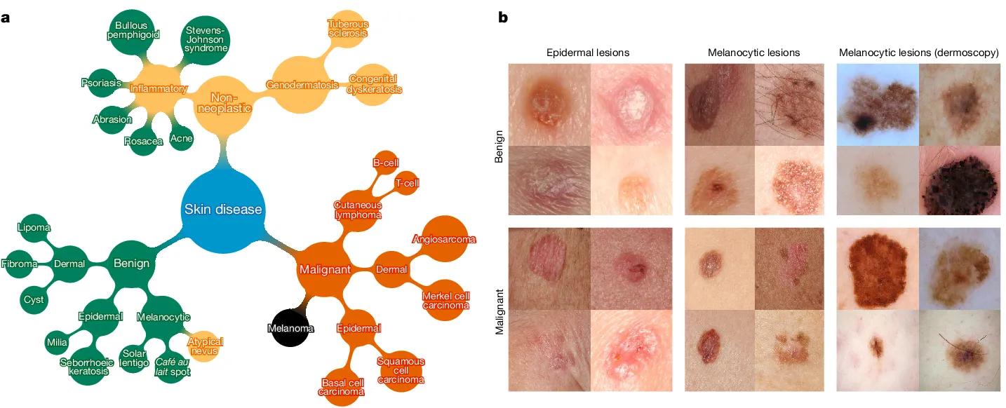
Table of Contents

1. Introduction
2. About Dataset
3. Use Cases of Skin Cancer Detection Model
4. Hands-on Tutorial
5. Conclusion
6. Frequently Asked Questions

Introduction

Skin cancer is a widespread and potentially life-threatening condition affecting millions worldwide. Timely detection significantly increases survival rates, and in this digital age, Convolutional Neural Networks (CNNs) have emerged as powerful allies in automating this process.

This blog serves as a detailed roadmap for ML Experts, ML Beginners and Product Managers, constructing a CNN model aimed at skin cancer detection, leveraging the HAM10000 dataset—a meticulously curated collection of skin lesion images. Beyond the technical nuances, this guide explores the transformative impact of integrating advanced technology, such as CNNs, into healthcare, particularly in the realm of dermatology.

By unraveling the intricacies of CNN implementation, this guide aims to empower both professionals and enthusiasts alike. Its objective is to illuminate the possibilities and implications of employing artificial intelligence to revolutionize skin cancer detection. Ultimately, this fusion of technology and healthcare seeks to expedite diagnosis, elevate patient care standards, and significantly impact global health outcomes.

About Dataset

The HAM10000 dataset is a significant compilation utilized for skin cancer classification, encompassing a diverse array of dermatoscopic images portraying various skin lesions categorized into distinct types of skin cancer.

Each image within this dataset is accompanied by crucial attributes such as age, gender, and localization, furnishing valuable information indispensable for analysis and classification tasks within the domain of dermatology.

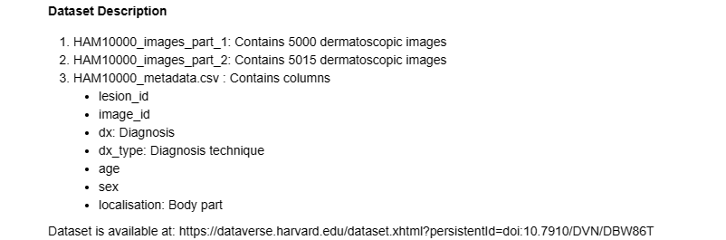
Key Dataset Components:

• HAM10000_images_part_1 and HAM10000_images_part_2: These folders house 5000 and 5015 dermatoscopic images, respectively.
• HAM10000_metadata.csv: This file contains columns like 'lesion_id', 'image_id', 'dx' (Diagnosis), 'dx_type' (Diagnosis technique), 'age', 'sex', and 'localization' (Body part).

Dataset Metrics and Details:

• Purpose and Composition: The dataset's objective is to facilitate neural network training for automated diagnosis of pigmented skin lesions. It consists of 10015 dermatoscopic images collected from different populations and modalities, showcasing a representative collection of key diagnostic categories: Actinic keratoses, Basal cell carcinoma, Melanoma, Nevi, and others.
• Ground Truth and Validation: Over 50% of the lesions are confirmed through histopathology. The remainder is verified through follow-up examination, expert consensus, or in-vivo confocal microscopy.
• Additional Data: For evaluation, the dataset includes test-set images and ground-truth data available as ISIC2018_Task3_Test_Images.zip and ISIC2018_Task3_Test_GroundTruth.csv, respectively.

Dataset Significance and Impact:

• Challenges and Research: The HAM10000 dataset served as a pivotal component for the ISIC 2018 challenge (Task 3), where test-set evaluations outperformed expert readers on an international scale.
• Additionally, it facilitated studies comparing human-computer collaboration scenarios, revealing the potential for improved diagnostic accuracy through machine learning augmentation.

Use Cases of Skin Cancer Detection Model

1. Early Detection and Improved Diagnosis

• Timely Intervention: CNN models can swiftly analyze dermatoscopic images, aiding in the early detection of malignant lesions.
• Accuracy and Precision: These models offer precise insights by identifying subtle patterns and features, potentially reducing missed diagnoses or false positives.

2. Tele-Dermatology and Remote Healthcare

• Remote Consultation: CNN models enable remote diagnosis by allowing dermatologists to assess skin lesions remotely, bridging the gap in areas lacking specialized medical professionals.
• Enhanced Accessibility: Patients in remote or underserved areas can receive expert evaluations without the need for physical appointments, improving access to healthcare services.

3. Augmenting Dermatologist's Expertise

• Decision Support System: CNN models act as a supportive tool, providing dermatologists with additional information and analysis to aid in their decision-making process.
• Reduced Workload: By automating routine tasks like lesion assessment, these models allow dermatologists to focus more on complex cases, optimizing their efficiency.

4. Personalized Treatment Plans

• Tailored Interventions: CNN models, by classifying lesions accurately, contribute to personalized treatment strategies based on the specific diagnosis and characteristics of the skin lesion.
• Prognosis Prediction: Predictive models based on CNN analyses can assist in predicting the likelihood of malignancy, aiding in designing individualized care plans.

5. Education and Training

• Training and Education: These models serve as valuable educational tools for medical students, residents, and practitioners, providing case-based learning and improving diagnostic skills.
• Continuous Learning: CNN models continuously learn from new data, enhancing their capabilities and staying updated with evolving diagnostic patterns.

Hands-on Tutorial

Outline

1. Importing Libraries
2. Loading and Understanding the Dataset
3. Creating a Dictionary for Image Path and Lesion Type
4. Exploratory Data Analysis (EDA)
5. Preprocessing
6. Data Augmentation
7. Model Creation, Training, and Testing
8. Evaluation and Testing of Models
9. Plotting Model Training Curve and Testing

1. Importing Libraries

This section imports essential libraries like NumPy, Pandas, TensorFlow, and PIL (Python Imaging Library). These libraries are crucial for data manipulation, image processing, machine learning model building, and evaluation.

# Importing Libraries
import os
import numpy as np
import pandas as pd

from PIL import Image
from glob import glob

from sklearn.preprocessing import LabelEncoder, StandardScaler

import plotly.graph_objects as go
import plotly.express as px
from plotly.subplots import make_subplots
import matplotlib.pyplot as plt
import pydot

from sklearn.model_selection import train_test_split
from sklearn.metrics import classification_report

import tensorflow as tf
from tensorflow.keras.preprocessing.image import ImageDataGenerator
from tensorflow.keras.models import Sequential
from tensorflow.keras.layers import Conv2D, Flatten, BatchNormalization, 
Dropout, Dense, MaxPool2D
from tensorflow.keras.callbacks import ReduceLROnPlateau, EarlyStopping

from IPython.display import display

2. Loading and Understanding the Dataset

It sets the directory path and loads the metadata CSV file containing information about the skin lesion dataset, utilizing Pandas' read_csv function.

# Setting data directory
data_directory = os.path.join("/kaggle/input/", "skin-cancer-mnist-ham10000/")
os.listdir(data_directory)

# Loading HAM10000_meatdata.csv 
data = pd.read_csv(os.path.join(data_directory, 'HAM10000_metadata.csv'))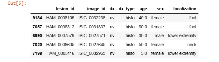

3. Creating a Dictionary for Image Path and Lesion Type

This code creates dictionaries to map image IDs to their file paths and lesion types for further data mapping and augmentation.

# Creating dictionary for image path, and lesion type
# Adding images from both the folders
imageid_path_dict = {os.path.splitext(os.path.basename(x))[0]: x
                     for x in glob(os.path.join(data_directory, '*', '*.jpg'))}

lesion_type_dict = {
    'nv': 'Melanocytic nevi (nv)',
    'mel': 'Melanoma (mel)',
    'bkl': 'Benign keratosis-like lesions (bkl)',
    'bcc': 'Basal cell carcinoma (bcc)',
    'akiec': 'Actinic keratoses (akiec)',
    'vasc': 'Vascular lesions (vasc)',
    'df': 'Dermatofibroma (df)'
}
label_mapping = {
    0: 'nv',
    1: 'mel',
    2: 'bkl',
    3: 'bcc',
    4: 'akiec',
    5: 'vasc',
    6: 'df'
}
reverse_label_mapping = dict((value, key) for key, value in label_mapping.items())

# Adding cell_type and image_path columns
data['cell_type'] = data['dx'].map(lesion_type_dict.get)
data['path'] = data['image_id'].map(imageid_path_dict.get)

%%time
# Adding image pixels
data['image_pixel'] = data['path'].map(lambda x: np.asarray(Image.open(x).resize((28,28))))

data.sample(5)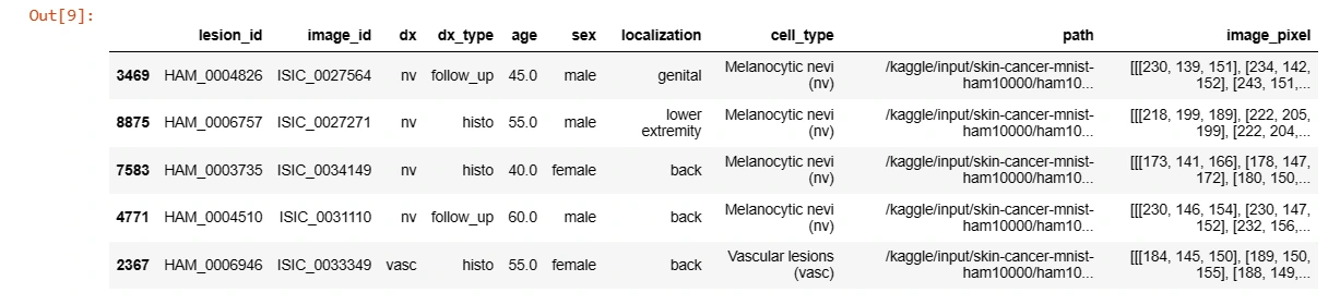

4. Exploratory Data Analysis (EDA)

The code generates subplots for visualizing various attributes of the dataset such as gender distribution, age, lesion types, and their respective counts using Plotly and Matplotlib.

fig = make_subplots(rows=2, cols=2,
                    subplot_titles=['Sex', 'Localisation', 'Age', 'Skin Type'],
                    vertical_spacing=0.15,
                    column_widths=[0.4, 0.6])

fig.add_trace(go.Bar(
            x=data['sex'].value_counts().index, 
            y=data['sex'].value_counts()),
            row=1, col=1)
fig.add_trace(go.Bar(
            x=data['localization'].value_counts().index, 
            y=data['localization'].value_counts()),
            row=1, col=2)
fig.add_trace(go.Histogram(
            x=data['age']),
            row=2, col=1)
fig.add_trace(go.Bar(
            x=data['dx'].value_counts().index.map(lesion_type_dict.get), 
            y=data['dx'].value_counts()),
            row=2, col=2)

for i in range(4):
    fig.update_yaxes(title_text='Count', row=i//2+1, col=i%2+1)
fig.update_layout(title='Distribution of Data', height=800)

fig.show()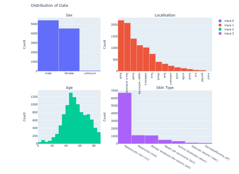

The code snippet below groups skin lesion images by their diagnosis labels ('dx'). For each label, it selects the first two images, displaying them in a grid of subplots. Using Matplotlib, it exhibits these images alongside their corresponding cell type labels, offering a visual representation of skin lesion samples categorized by diagnosis labels for quick inspection and comparison.

# Displaying 2 images for each label
sample_data = data.groupby('dx').apply(lambda df: df.iloc[:2, [9, 7]])
plt.figure(figsize=(22, 32))
for i in range(14):
    plt.subplot(7, 5, i + 1)
    plt.imshow(np.squeeze(sample_data['image_pixel'][i]))
    img_label = sample_data['cell_type'][i]
    plt.title(img_label)
    plt.axis("off")
plt.show()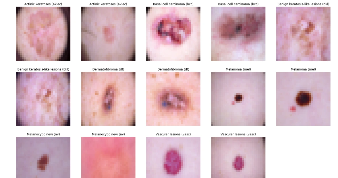

5. Preprocessing

Null values in the 'age' column are filled with the mean age and converted to integers. The 'label' column is created by mapping lesion types to numerical values for classification.

data.info()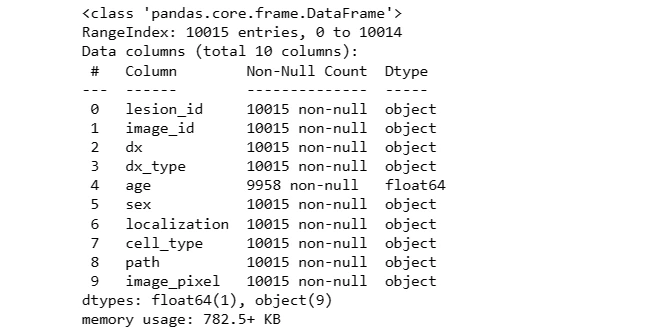

# Checking null values
data.isnull().sum()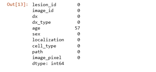

# Handling null values
data['age'].fillna(value=int(data['age'].mean()), inplace=True)
# Converting dtype of age to int32
data['age'] = data['age'].astype('int32')

# Categorically encoding label of the images 
data['label'] = data['dx'].map(reverse_label_mapping.get)

data.sample(5)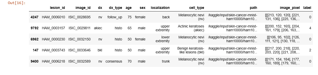

6. Data Augmentation

This section augments the data by oversampling different classes, aiming to balance the dataset. It then combines the original and augmented data to create a more robust dataset for training.

data = data.sort_values('label')
data = data.reset_index()

%%time
index1 = data[data['label'] == 1].index.values
index2 = data[data['label'] == 2].index.values
index3 = data[data['label'] == 3].index.values
index4 = data[data['label'] == 4].index.values
index5 = data[data['label'] == 5].index.values
index6 = data[data['label'] == 6].index.values

df_index1 = data.iloc[int(min(index1)):int(max(index1)+1)]
df_index2 = data.iloc[int(min(index2)):int(max(index2)+1)]
df_index3 = data.iloc[int(min(index3)):int(max(index3)+1)]
df_index4 = data.iloc[int(min(index4)):int(max(index4)+1)]
df_index5 = data.iloc[int(min(index5)):int(max(index5)+1)]
df_index6 = data.iloc[int(min(index6)):int(max(index6)+1)]

df_index1 = df_index1.append([df_index1]*4, ignore_index = True)
df_index2 = df_index2.append([df_index2]*4, ignore_index = True)
df_index3 = df_index3.append([df_index3]*11, ignore_index = True)
df_index4 = df_index4.append([df_index4]*17, ignore_index = True)
df_index5 = df_index5.append([df_index5]*45, ignore_index = True)
df_index6 = df_index6.append([df_index6]*52, ignore_index = True)

frames = [data, df_index1, df_index2, df_index3, df_index4, df_index5, df_index6]
final_data = pd.concat(frames)

%%time
print(data.shape)
print(final_data.shape)

fig = make_subplots(rows=2, cols=2,
                    subplot_titles=['Sex', 'Localisation', 'Age', 'Skin Type'],
                    vertical_spacing=0.15,
                    column_widths=[0.4, 0.6])

fig.add_trace(go.Bar(
            x=final_data['sex'].value_counts().index, 
            y=final_data['sex'].value_counts()),
            row=1, col=1)
fig.add_trace(go.Bar(
            x=final_data['localization'].value_counts().index, 
            y=final_data['localization'].value_counts()),
            row=1, col=2)
fig.add_trace(go.Histogram(
            x=final_data['age']),
            row=2, col=1)
fig.add_trace(go.Bar(
            x=final_data['dx'].value_counts().index.map(lesion_type_dict.get), 
            y=final_data['dx'].value_counts()),
            row=2, col=2)

for i in range(4):
    fig.update_yaxes(title_text='Count', row=i//2+1, col=i%2+1)
fig.update_layout(title='Distribution of Data after augmentation', height=800)

fig.show()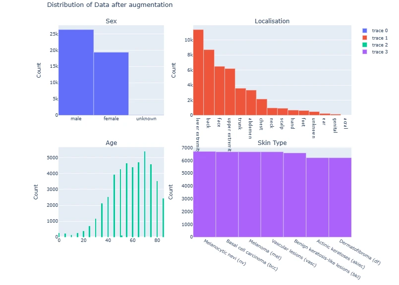

Creating 2 sets of data for Model Training and Testing

Original Data: Without solving the class imbalance problem

Augmented Data: After solving the class imbalance problem

# ORIGINAL DATA
# Converting image pixel columnm into required format
X_orig = data['image_pixel'].to_numpy()
X_orig = np.stack(X_orig, axis=0)
Y_orig = np.array(data.iloc[:, -1:])
print(X_orig.shape)
print(Y_orig.shape)

(10015, 28, 28, 3)
(10015, 1)

# AUGMENTED DATA
# Converting image pixel columnm into required format
X_aug = final_data['image_pixel'].to_numpy()
X_aug = np.stack(X_aug, axis=0)
Y_aug = np.array(final_data.iloc[:, -1:])
print(X_aug.shape)
print(Y_aug.shape)

(45756, 28, 28, 3)
(45756, 1)

7. Model Creation, Training, and Testing

This code snippet defines a sequential model architecture using Convolutional (Conv2D) and Pooling (MaxPool2D) layers along with fully connected (Dense) layers for classification. It compiles the model with an optimizer and loss function for training.

For Original Data:

%%time
def prepare_for_train_test(X, Y):
    # Splitting into train and test set
    X_train, X_test, Y_train, Y_test = train_test_split(X, Y, test_size=0.2, random_state=1)
    
    # Prepare data for training and testing the model
    train_datagen = ImageDataGenerator(rescale = 1./255,
                                  rotation_range = 10,
                                  width_shift_range = 0.2,
                                  height_shift_range = 0.2,
                                  shear_range = 0.2,
                                  horizontal_flip = True,
                                  vertical_flip = True,
                                  fill_mode = 'nearest')
    train_datagen.fit(X_train)
    test_datagen = ImageDataGenerator(rescale = 1./255)
    test_datagen.fit(X_test)
    return X_train, X_test, Y_train, Y_test

def create_model():
    model = Sequential()
    model.add(Conv2D(16, kernel_size = (3,3), input_shape = (28, 28, 3), 
    activation = 'relu', padding = 'same'))
    model.add(MaxPool2D(pool_size = (2,2)))

    model.add(Conv2D(32, kernel_size = (3,3), activation = 'relu', padding = 'same'))
    model.add(MaxPool2D(pool_size = (2,2), padding = 'same'))

    model.add(Conv2D(64, kernel_size = (3,3), activation = 'relu', padding = 'same'))
    model.add(MaxPool2D(pool_size = (2,2), padding = 'same'))
    model.add(Conv2D(128, kernel_size = (3,3), activation = 'relu', padding = 'same'))
    model.add(MaxPool2D(pool_size = (2,2), padding = 'same'))

    model.add(Flatten())
    model.add(Dense(64, activation = 'relu'))
    model.add(Dense(32, activation='relu'))
    model.add(Dense(7, activation='softmax'))

    optimizer = tf.keras.optimizers.Adam(learning_rate = 0.001)

    model.compile(loss = 'sparse_categorical_crossentropy',
                 optimizer = optimizer,
                  metrics = ['accuracy'])
    print(model.summary())
#     tf.keras.utils.plot_model(model, to_file="model.png")
    return model;

def train_model(model, X_train, Y_train, EPOCHS=25):
    early_stop = EarlyStopping(monitor='val_loss', patience=10, verbose=1, 
                           mode='auto', restore_best_weights=True)
    
    reduce_lr = ReduceLROnPlateau(monitor='val_loss', factor=0.1, patience=5, 
                              verbose=1, mode='auto')
    
    history = model.fit(X_train,
                        Y_train,
                        validation_split=0.2,
                        batch_size = 64,
                        epochs = EPOCHS,
                        callbacks = [reduce_lr, early_stop])
    return history
    
def plot_model_training_curve(history):
    fig = make_subplots(rows=1, cols=2, subplot_titles=['Model Accuracy', 'Model Loss'])
    fig.add_trace(
        go.Scatter(
            y=history.history['accuracy'], 
            name='train_acc'), 
        row=1, col=1)
    fig.add_trace(
        go.Scatter(
            y=history.history['val_accuracy'], 
            name='val_acc'), 
        row=1, col=1)
    fig.add_trace(
        go.Scatter(
            y=history.history['loss'], 
            name='train_loss'), 
        row=1, col=2)
    fig.add_trace(
        go.Scatter(
            y=history.history['val_loss'], 
            name='val_loss'), 
        row=1, col=2)
    fig.show()
    
def test_model(model, X_test, Y_test):
    model_acc = model.evaluate(X_test, Y_test, verbose=0)[1]
    print("Test Accuracy: {:.3f}%".format(model_acc * 100))
    y_true = np.array(Y_test)
    y_pred = model.predict(X_test)
    y_pred = np.array(list(map(lambda x: np.argmax(x), y_pred)))
    clr = classification_report(y_true, y_pred, target_names=label_mapping.values())
    print(clr)
    
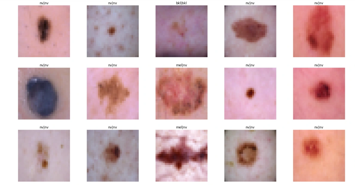
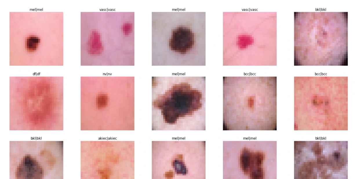
    sample_data = X_test[:15]
    plt.figure(figsize=(22, 12))
    for i in range(15):
        plt.subplot(3, 5, i + 1)
        plt.imshow(sample_data[i])
        plt.title(label_mapping[y_true[i][0]] + '|' + label_mapping[y_pred[i]])
        plt.axis("off")
    plt.show() 

# For Original Dataset
X_train_orig, X_test_orig, Y_train_orig, Y_test_orig = prepare_for_train_test(X_orig, Y_orig)

model1 = create_model()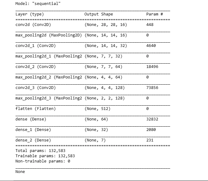

model1_history = train_model(model1, X_train_orig, Y_train_orig, 50)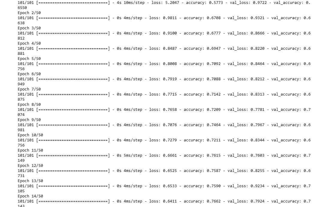

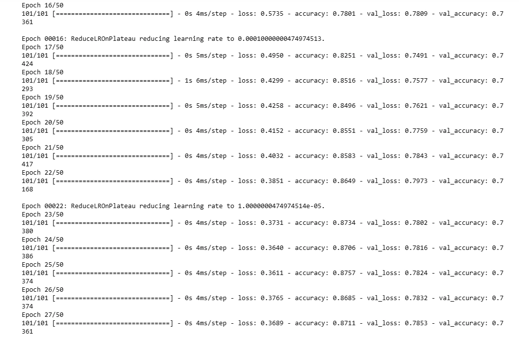
For Augmented Dataset:

# For Augmented Dataset
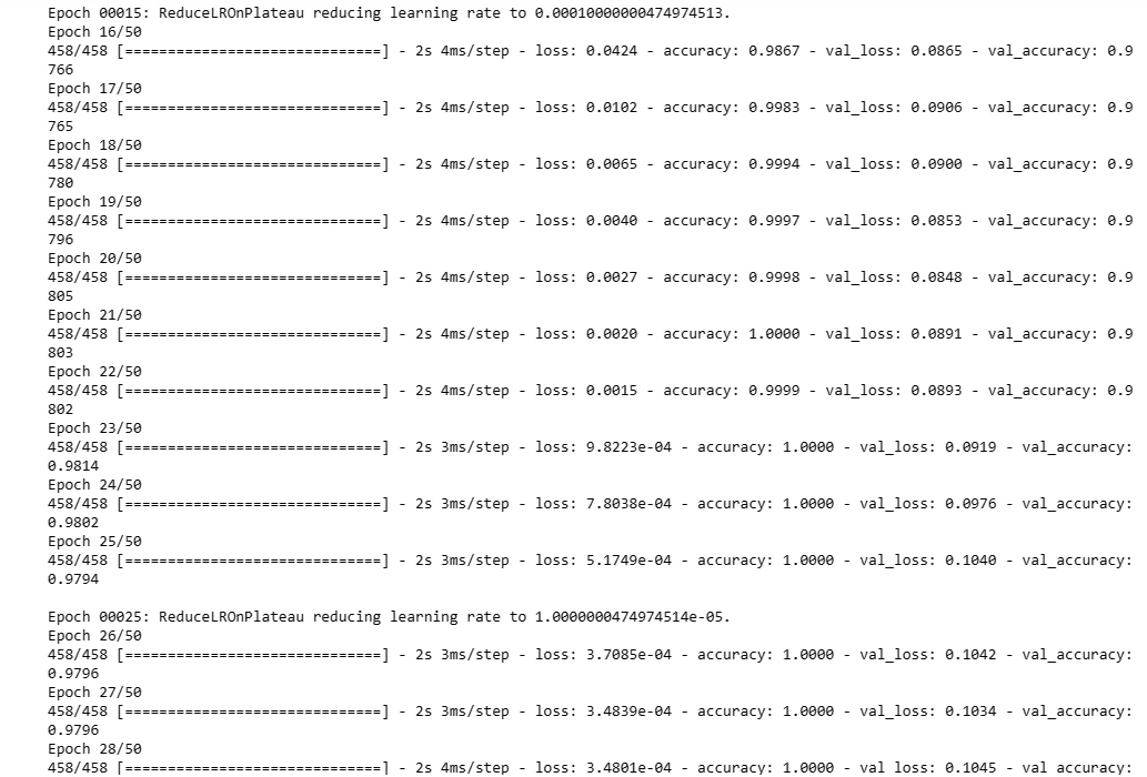
X_train_aug, X_test_aug, Y_train_aug, Y_test_aug = prepare_for_train_test(X_aug, Y_aug)

model2 = create_model()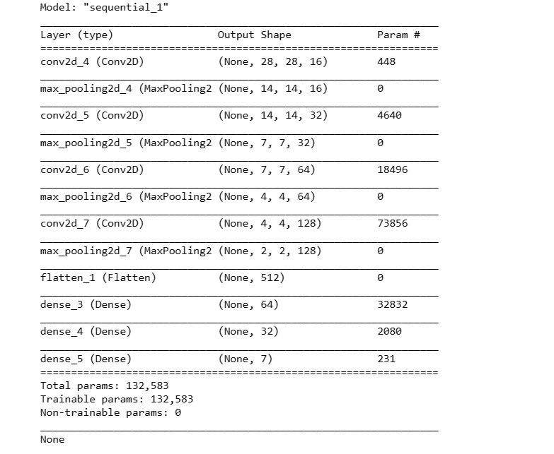

model2_history = train_model(model2, X_train_aug, Y_train_aug, 50)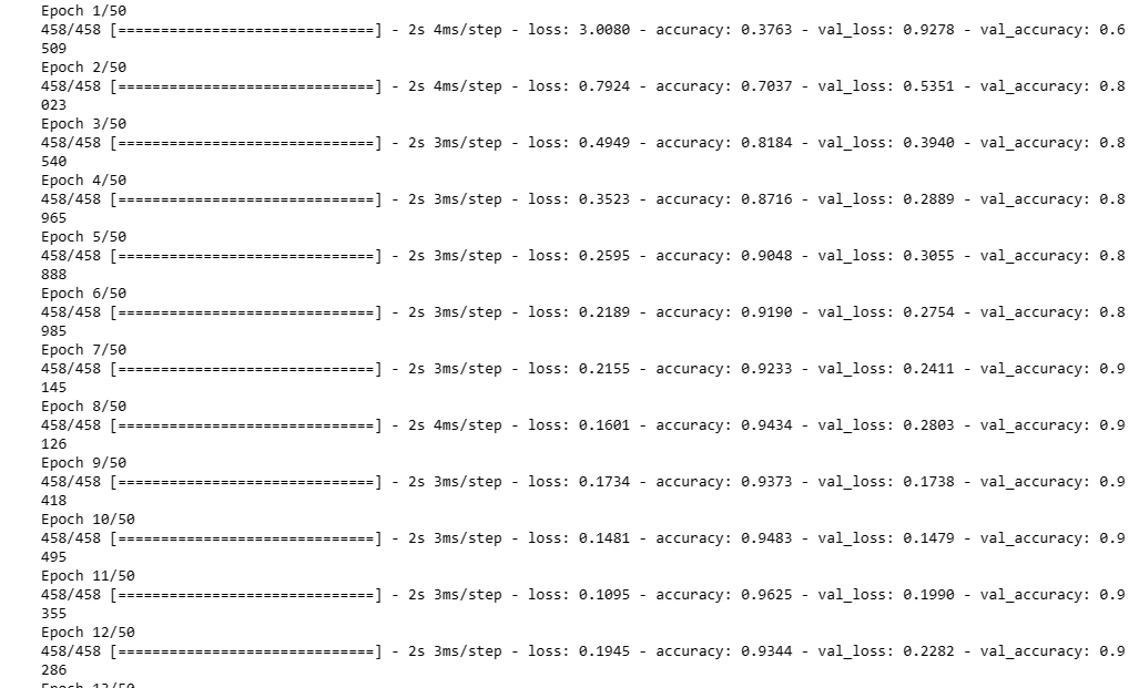

8. Evaluation and Testing of Models

The code snippet evaluates the performance of the neural network model 'model1' on a separate test dataset ('X_test_orig') and corresponding labels ('Y_test_orig').

It calculates the model's accuracy on the test data and generates a classification report, showcasing the model's predictive capability and its agreement with the ground truth labels for skin lesion classification.

For Original Dataset:

test_model(model1, X_test_orig, Y_test_orig)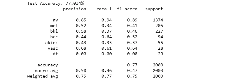

For Augmented Dataset:

test_model(model2, X_test_aug, Y_test_aug)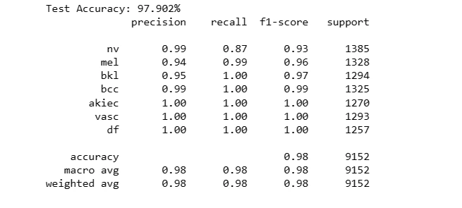

9. Plotting Model Training Curve and Testing

This section visualizes the model's performance by plotting training and validation accuracy/loss over epochs. Additionally, it evaluates the trained model on test data, displaying sample predictions versus true labels.

For Original Dataset:

plot_model_training_curve(model1_history)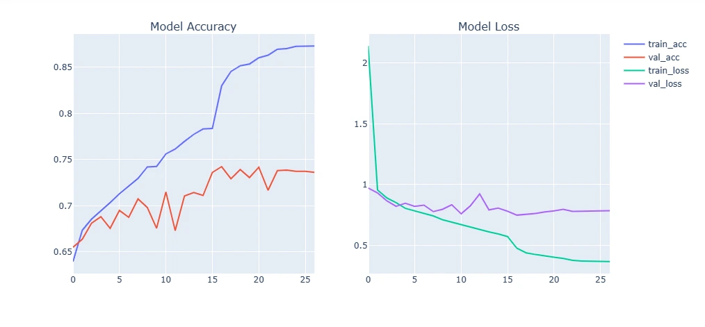

For Augmented Dataset:

plot_model_training_curve(model2_history)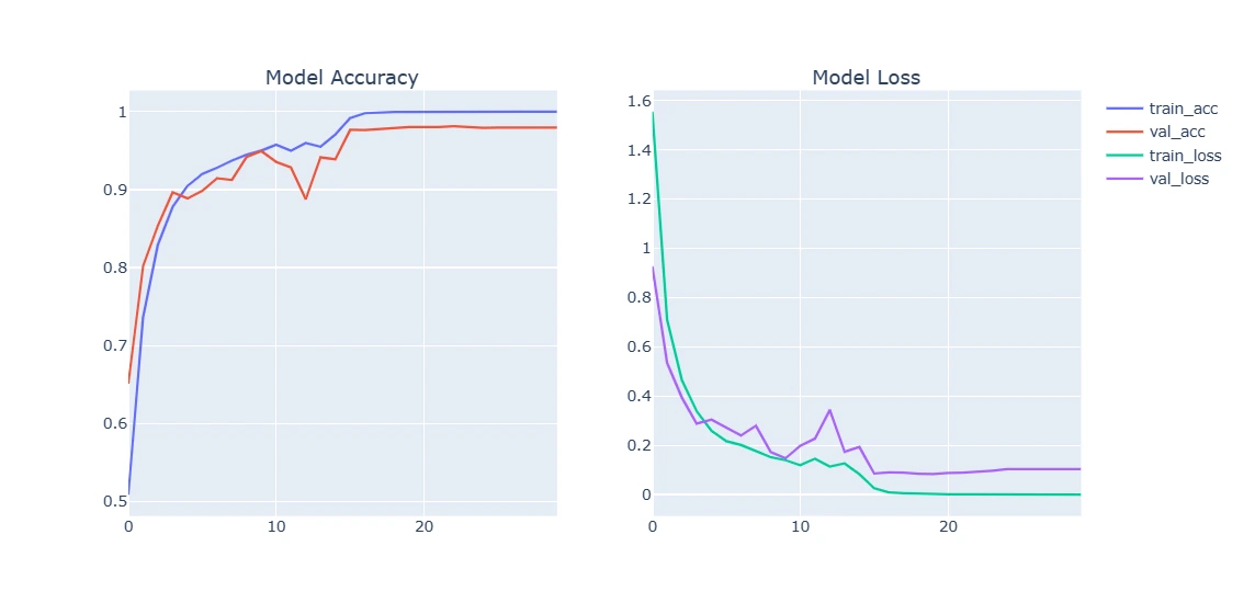

Conclusion

This blog extensively covered the process of building a CNN model for skin cancer detection. It emphasized the importance of early detection and how AI-powered models can assist dermatologists in accurate diagnosis. Additionally, leveraging CNNs for skin cancer detection showcases the potential of technology in healthcare, especially in aiding medical professionals for timely interventions.

Frequently Asked Questions

1. Can convolutional neural networks detect skin cancer?

Yes, convolutional neural networks (CNNs) have demonstrated remarkable capability in detecting skin cancer. By analyzing and learning from vast datasets of dermatological images, CNNs can effectively identify patterns and features indicative of various skin conditions, including melanoma and other types of skin cancer.

These networks excel in recognizing irregularities in moles or lesions, leveraging their ability to extract hierarchical features from images and classify them based on learned patterns. Their accuracy in detecting skin cancer has shown promising results comparable to or even surpassing that of trained dermatologists, showcasing their potential as a valuable tool in early diagnosis and improving healthcare outcomes for patients.

2. What are Ann-based skin cancer detection techniques?

Artificial Neural Network (ANN)-based approaches for skin cancer detection encompass methods that use neural networks to analyze dermatological images. Specifically, Convolutional Neural Networks (CNNs) have gained prominence for their effectiveness in recognizing skin cancer patterns. These techniques involve CNNs processing images through layers that extract relevant features, trained on datasets to identify textures and structures indicative of different skin conditions.

Additionally, ANN-based methods may incorporate techniques like Statistical Region Merging (SRM) or Gray Level Co-occurrence Matrix (GLCM) for enhanced feature extraction. Backpropagation Neural Networks (BPNNs), a type of ANN, are commonly employed to classify skin lesions into cancerous or non-cancerous categories based on learned features.

Overall, these ANN-based approaches utilize CNNs, BPNNs, and various image processing methods to aid in accurate skin cancer diagnosis from medical images.

3. Do neural networks learn to account for skin color?

Yes, neural networks can learn to account for skin color as part of their training process. When dealing with skin cancer detection, neural networks are trained on diverse datasets that include images of various skin tones and colors. While the emphasis in many studies may be on discerning whether an image contains cancerous lesions or not, neural networks inherently learn to recognize and factor in different skin colors as they analyze and process these images.

However, it's important to note that the primary focus of most studies might be on lesion identification rather than pinpointing specific symptoms of skin cancer on various parts of the body in response to patient inquiries.

Nonetheless, the neural networks' training on diverse skin tones equips them to detect anomalies or patterns related to skin cancer across different skin colors, aiding in their ability to identify potential issues in various populations.

Looking for high quality training data to train your skin cancer detection model? Talk to our team to get a tool demo.