ML Hands-On Guide on Kitsune-Network Attack Detection

Introduction

In today's digital world of cybersecurity, the threat is ever-evolving, necessitating robust defense mechanisms to safeguard against malicious activities.

Kitsune, a neural network-based Network Intrusion Detection System (NIDS), emerges as a cutting-edge solution to this pressing challenge.

By harnessing the power of deep learning techniques like Convolutional Neural Networks (CNNs), Long Short-Term Memory (LSTM), and Gated Recurrent Units (GRUs), Kitsune autonomously learns patterns indicative of cyber attacks within network traffic.

Its role and significance in security and surveillance are paramount, offering proactive defense measures and the ability to detect novel attack vectors in real time.

This blog serves as a comprehensive guide and hands-on tutorial, catering to ML experts, beginners, product managers, researchers, and cybersecurity professionals by providing valuable insights into Kitsune's capabilities and practical applications in enhancing network security.

Hands-On Tutorial

1. Import Libraries

Import necessary libraries for data manipulation (numpy, pandas), data visualization (seaborn, matplotlib).

import numpy as np
import pandas as pd

import seaborn as sns
import matplotlib.pyplot as plt

2. Column Names

Define column names for the dataset.

colnames = ["1", "2", "3", "4", "5", "6", "7", "8", "9", "10", "11", "12", "13", "14", "15", "16", "17", "18", "19", "20", "21", "22", "23", "24", "25", "26", "27", "28", "29", "30", "31", "32", "33", "34", "35", "36", "37", "38", "39", "40", "41", "42", "43", "44", "45", "46", "47", "48", "49", "50", "51", "52", "53", "54", "55", "56", "57", "58", "59", "60", "61", "62", "63", "64", "65", "66", "67", "68", "69", "70", "71", "72", "73", "74", "75", "76", "77", "78", "79", "80", "81", "82", "83", "84", "85", "86", "87", "88", "89", "90", "91", "92", "93", "94", "95", "96", "97", "98", "99", "100", "101", "102", "103", "104", "105", "106", "107", "108", "109", "110", "111", "112", "113", "114", "115"]

3. Read CSV and Display Information

Read the CSV file into a data frame using the specified column names.

Display information about the data frame (info()).

Display the first five rows of the data frame (head()).

#read csv, using data training
df = pd.read_csv('/kaggle/input/network-attack-dataset-kitsune/ARP MitM/ARP_MitM_dataset.csv', names=colnames, header=None)
df.info()
df.head()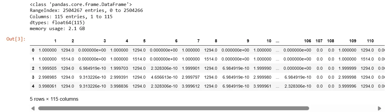

4. Unique Values in DataFrame

Display the number of unique values in each column of the DataFrame.

df.nunique()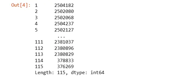

5. Read Labels CSV and Display Information

Read the labels CSV file into dataset_label DataFrame.

Display information about the labels DataFrame.

Print value counts for the 'x' column.

dataset_label = pd.read_csv('/kaggle/input/network-attack-dataset-kitsune/ARP MitM/ARP_MitM_labels.csv', dtype={"": int, "x": 'float64'})
dataset_label.info()
print('=====Labels=========')
print(dataset_label.x.value_counts())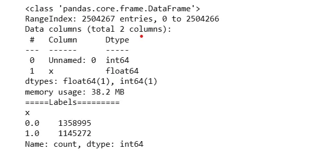

6. Data Preprocessing - Standard Scaling

Extract values from the DataFrame and store them in best_features.

Import StandardScaler from sci-kit-learn and scale the data.

Print the preprocessed data.

best_features=df.values
from sklearn.preprocessing import StandardScaler
sc_x=StandardScaler()
df_pre=sc_x.fit_transform(best_features)
print('=====Data Preprocessing=========')
print(df_pre)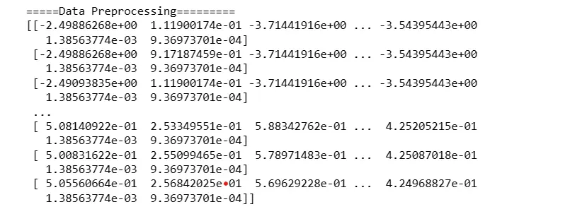

7. Train-Test Split

Split the data into training and testing sets.

from sklearn.model_selection import train_test_split
y=dataset_label["x"]
y=np.ravel(y)
print(df_pre.shape)
print(y.shape)
X_train, X_test, Y_train, Y_test = train_test_split(df_pre, y, test_size =0.2)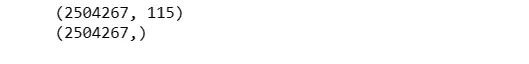

8. Neural Network Model (LSTM, GRU, Dense)

Define a neural network model using LSTM, GRU, and Dense layers.

Compile the model with a specified optimizer, loss function, and metrics.

Train the model and save it.

from keras.models import Sequential
from keras.layers import Flatten, Dense, Conv1D, MaxPool1D, Dropout,LeakyReLU,GRU,LSTM,Concatenate,BatchNormalization,Bidirectional,Input
from sklearn.metrics import accuracy_score, precision_score, recall_score, f1_score
from keras.models import Sequential
from sklearn.metrics import accuracy_score
from sklearn.metrics import roc_curve,roc_auc_score
from sklearn.model_selection import StratifiedKFold
from collections import Counter
from sklearn import metrics
import itertools

def plot_confusion_matrix(cm, classes,
                          normalize=False,
                          title='Confusion matrix',
                          cmap=plt.cm.Blues):

    plt.imshow(cm, interpolation='nearest', cmap=cmap)
    plt.title(title)
    plt.colorbar()
    tick_marks = np.arange(len(classes))
    plt.xticks(tick_marks, classes, rotation=45)
    plt.yticks(tick_marks, classes)

    if normalize:
        cm = cm.astype('float') / cm.sum(axis=1)[:, np.newaxis]
        print("Normalized confusion matrix")
    else:
        print('Confusion matrix, without normalization')

    thresh = cm.max() / 2.
    for i, j in itertools.product(range(cm.shape[0]), range(cm.shape[1])):
        plt.text(j, i, cm[i, j],
                 horizontalalignment="center",
                 color="white" if cm[i, j] > thresh else "black")

    plt.tight_layout()
    plt.ylabel('True label')
    plt.xlabel('Predicted label')

from sklearn.discriminant_analysis import LinearDiscriminantAnalysis
from sklearn.datasets import load_digits
from sklearn.model_selection import cross_val_predict
from sklearn.metrics import f1_score
from sklearn.metrics import confusion_matrix, classification_report, precision_score
from sklearn import metrics
from sklearn.model_selection import train_test_split
AX_train=X_train
AX_test=X_test
AY_train=Y_train
AY_test=Y_test
X_train1 = np.array(X_train).reshape(X_train.shape[0], X_train.shape[1], 1)
X_test1 = np.array(X_test).reshape(X_test.shape[0], X_test.shape[1], 1)
model = Sequential()
model.add(LSTM(50, input_shape=(X_train.shape[1],1), return_sequences=True))
model.add(GRU(50, return_sequences=True))
model.add(GRU(50)) 
model.add(Dense(units = 2, activation='softmax'))
model.compile(optimizer='adam', loss = 'sparse_categorical_crossentropy', metrics=['accuracy'])
model_history = model.fit(X_train1, Y_train, epochs=2, batch_size = 128, validation_data = (X_test1, Y_test))
model.save('LSTM_GRU.h5')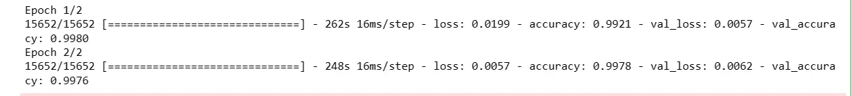

9. Model Evaluation

Evaluate the model on the test set.

Calculate and print various metrics.

from sklearn.metrics import accuracy_score
import time
y_true=Y_test
start_time = time.time()
y_predict=model.predict(X_test1)
y_predict=np.argmax(y_predict,axis=1)
end_time = time.time()
Hybrid_testing_time = end_time - start_time

10. Confusion Matrix Plotting Function

Define a function to plot a confusion matrix.

from sklearn.metrics import classification_report,confusion_matrix,accuracy_score,precision_recall_fscore_support
from sklearn.metrics import f1_score,roc_auc_score
test_accuracy=accuracy_score(y_true, y_predict)
precision,recall,fscore,none= precision_recall_fscore_support(y_true, y_predict, average='weighted')
# print(classification_report(y_true,y_predict))
cm = metrics.confusion_matrix(y_true,y_predict)
plot_confusion_matrix(cm, classes=['not malicous', 'malicous'])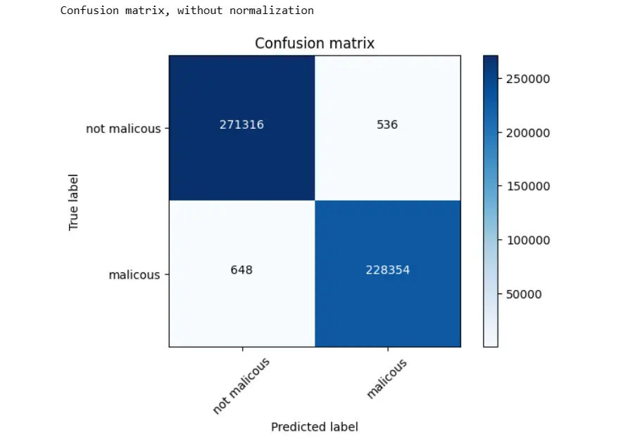

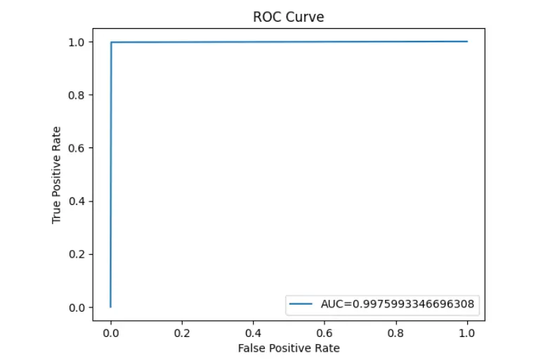
11. ROC Curve and Model Accuracy/Precision/Recall/ F1 Score

Plot the Receiver Operating Characteristic (ROC) curve.

fpr, tpr, _ = roc_curve(y_true,y_predict)
auc = roc_auc_score(y_true,y_predict)
from sklearn.metrics import matthews_corrcoef
conf = confusion_matrix(y_true,y_predict)
TN = conf[0][0]
FN = conf[1][0]
TP = conf[1][1]
FP = conf[0][1]
TNR = TN / (TN + FP)
MCC = matthews_corrcoef(y_true,y_predict)
NPV = TN / (TN + FN)
FDR = FP / (FP + TP)
FNR = FN / (FN + TP)
FOR = FN / (FN + TN)
FPR = FP / (FP + TN)
print('Accuracy of CNN-GRU-LSTM: '+ str(test_accuracy))
print('Precision of CNN-GRU-LSTM: '+(str(precision)))
print('Recall of CNN-GRU-LSTM: '+(str(recall)))
print('F1-score of CNN-GRU-LSTM: '+(str(fscore)))
print("True Negative Rate (TNR):", TNR)
print("Matthew's Correlation Coefficient (MCC):", MCC)
print("Negative Predictive Value (NPV):", NPV)
print("False Discovery Rate (FDR):", FDR)
print("False Negative Rate (FNR):", FNR)
print("False Omission Rate (FOR):", FOR)
print("False Positive Rate (FPR):", FPR)
print(f"Testing time: {Hybrid_testing_time} seconds")
#create ROC curve
plt.plot(fpr,tpr,label="AUC="+str(auc))
plt.ylabel('True Positive Rate')
plt.xlabel('False Positive Rate')
plt.legend(loc=4)
plt.title('ROC Curve')
plt.show()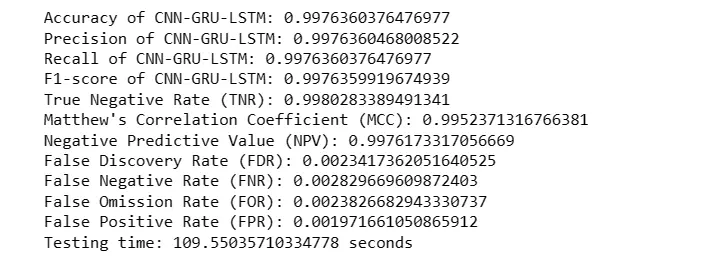

12. SHAP Values

Import SHAP library and calculate SHAP values.

import shap
explainer = shap.KernelExplainer(model,X_test[:50,:])
shap_values = explainer.shap_values(X_test[20,:], nsamples=500)

shap.initjs()
shap_values50 = explainer.shap_values(X_test[50:100,:], nsamples=500)

shap.summary_plot(shap_values50[0], X_test[50:100,:], show=True)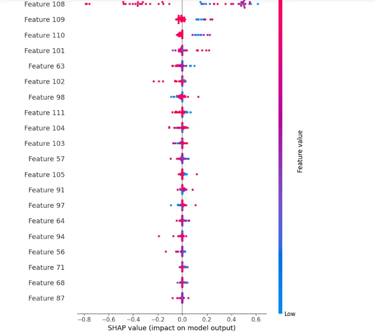

Conclusion

In this blog, we've explored Kitsune, a powerful tool for keeping computer networks safe from cyber threats.

By using advanced math and learning from past data, Kitsune can spot suspicious activity on its own, without needing constant supervision.

We've also gone through a hands-on tutorial, showing how to use Kitsune to analyze network data and build a model to detect attacks.

Whether you're new to cybersecurity or an expert, Kitsune offers valuable insights and practical applications for enhancing network security.

With its ability to adapt to new threats in real-time, Kitsune is a valuable asset in the ongoing battle against cybercrime.

Frequently Asked Questions

1. What is kitsune neural network based NIDS?

Kitsune is a neural network-based Network Intrusion Detection System (NIDS) that utilizes a combination of deep learning techniques, specifically Convolutional Neural Networks (CNNs), Long Short-Term Memory (LSTM), and Gated Recurrent Units (GRUs).

It aims to detect malicious activities within network traffic by learning patterns indicative of attacks.

Kitsune preprocesses network data, trains a neural network model on the preprocessed data, and then uses the trained model to classify network traffic as either malicious or benign.

Its architecture enables it to adapt to evolving attack strategies and effectively detect previously unseen threats in real-time.

2. Can kitsune detect attacks on a local network without supervision?

Yes, Kitsune has the capability to detect attacks on a local network without supervision.

It achieves this through its use of unsupervised learning techniques, which enable it to identify anomalous patterns in network traffic without relying on labeled data or predefined attack signatures.

By leveraging deep learning architectures like CNNs, LSTMs, and GRUs, Kitsune can autonomously learn the normal behavior of the network and detect deviations from this baseline, flagging them as potential attacks.

This unsupervised approach allows Kitsune to adapt to emerging threats and detect novel attack patterns without requiring constant manual intervention or supervision.

Looking for high quality training data to train your vision/NLP models? Talk to our team to get a demo.