How to Build an End-to-End ML Pipeline

Machine learning pipeline refers to the complete workflow and processes of building and deploying a machine learning model. It automates and standardizes the workflow involved in creating a machine-learning model.

A machine learning pipeline consists of sequential steps, which include data extraction and preprocessing to model training and deployment. It is a central product for data science teams, incorporating best practices and enabling scalable execution.

Whether managing multiple models or frequently updating a single model, an end-to-end machine learning pipeline is essential for effective and efficient implementation.

The benefits of having an end-to-end machine-learning pipeline are many, some of which include the following:

1. Ensure reproducibility: By running the channel repeatedly on similar inputs, consistent outputs can be obtained, ensuring reproducibility and reliability in machine learning.
   
2. Simplify workflow: The pipeline automates multiple steps in the machine learning workflow. This reduces the need for manual intervention from the data science team, making the process more efficient and streamlined.
   
3. Accelerate deployment: The pipeline helps reduce the time data and models take to the production phase. This enables faster deployment of machine learning solutions and quicker integration into real-world applications.
   
4. Enable focus on innovation: With modular components and automation in place, the pipeline frees the data science team to focus more on developing new solutions rather than spending excessive time maintaining existing ones.
   
5. Facilitate reusability: The pipeline allows for easy reusability of components in the machine learning workflow. Specific steps can be reused to create and deploy end-to-end solutions seamlessly integrated with systems without starting from scratch each time.

Developing a primary end-to-end machine learning Pipeline

Sklearn offers a range of powerful methods for various machine learning steps, including Column Transformer, Standard Scaler, One-Hot Encoder, Simple Imputer, and more.

These methods provide convenient solutions for data scientists, simplifying their work processes.

While this article doesn't delve into a detailed explanation of each method to keep the reading time short, it highlights the usage of several models in building ML pipelines, as demonstrated in the example below.

Custom Machine Learning Pipeline

While Sklearn offers a wide range of models for building machine learning pipelines, such as Iterative Imputer, Normalizer, and Label Encoder, this article focuses explicitly on custom models.

The Sklearn website provides comprehensive documentation for these models, allowing users to explore their functionalities in detail.

To understand how to build a custom machine-learning pipeline, we take an example of the Bike sharing dataset, which is accessible for download here.

This dataset comprises information on the number of bikes rented during specific hours and other relevant features. Our objective is to construct a model that can forecast the number of bikes that will be rented using these features.

Data exploration and preprocessing

The consensus among most machine learning practitioners is that data exploration and preprocessing constitute a significant portion of their work.

This is because the available data often comes with challenges, such as incompleteness or an unsuitable format for direct usage.

First, we will import the necessary libraries and load the data into our notebook. This will enable us to perform the required data exploration and preprocessing tasks.

import numpy as np
import pandas as pd
import matplotlib.pyplot as plt
import seaborn as sns
from sklearn.model_selection import train_test_split
import math  
import sklearn.metrics  
from sklearn.linear_model import LinearRegression
from sklearn.ensemble import RandomForestRegressor
from sklearn.pipeline import Pipeline

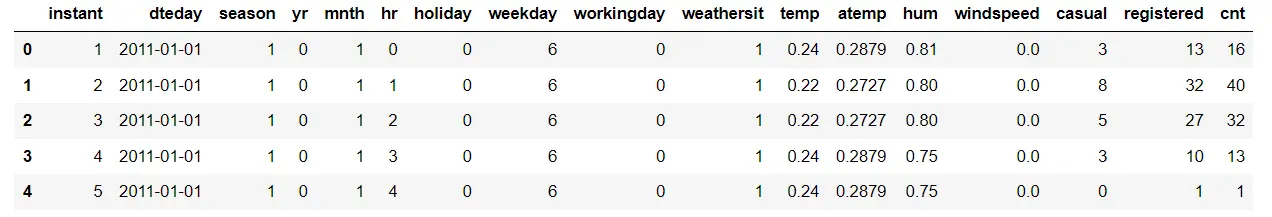
data = pd.read_csv('./Data/hour.csv')
data.head()

We can obtain a summary of the dataset by using the DataFrame.info() method from Pandas.

This method provides information about the column names, the number of non-null rows, and the data types of each column. This summary helps us understand the structure and characteristics of the dataset used.

data.info()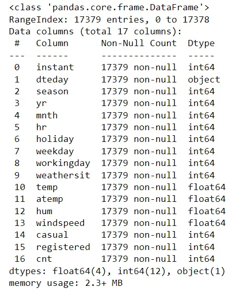

data.columns

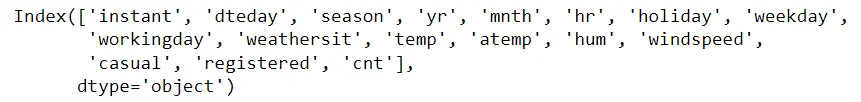
There are no missing values in the data. However, the column names could be more descriptive and readable. Let's rename the columns to make them more informative and easier to understand.

data.rename(columns = {'instant':'index', 'dteday':'datetime',
'yr':'year', 'mnth':'month', 'holiday':'is_holiday',
'workingday':'is_workingday','weathersit':'weather_conditions','hum':'humidity','hr':'hour', 'cnt':'count'}, inplace = True)

data.head()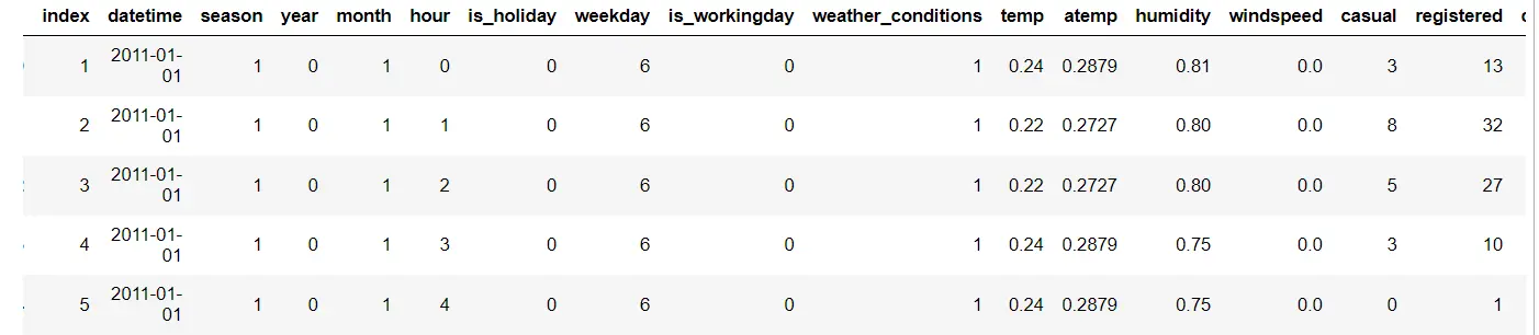

We excluded the 'record_id' column as it provided no valuable information regarding bike rentals.

Additionally, we combined the 'casual' and 'registered' columns into a single column called 'count' to avoid data leakage.

This precaution prevents the model from learning from information in the training data that may not be present in the test set. This ensures better performance when the model is deployed in production.

data.drop(['index','casual','registered'], axis = 1, inplace = True)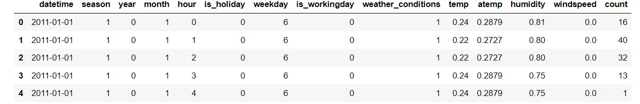

The columns in the dataset have different data types, and we need to convert them to the most suitable data type for each column. This ensures that the data is represented accurately and efficiently.

data['datetime'] = pd.to_datetime(data.datetime)
# categorical variables
data['season'] = data.season.astype('category')
data['is_holiday'] = data.is_holiday.astype('category')
data['weekday'] = data.weekday.astype('category')
data['weather_conditions'] = data.weather_conditions.astype('category')
data['is_workingday'] = data.is_workingday.astype('category')
data['month'] = data.month.astype('category')
data['year'] = data.year.astype('category')
data['hour'] = data.hour.astype('category')

plt.figure(figsize = (8,6))
sns.heatmap(data.corr(),annot = True, cmap = 'BrBG')

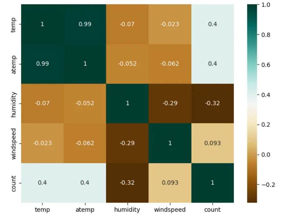
        Figure: Heatmap for feature correlation

To mitigate the issue of multicollinearity, we have decided to remove the 'atemp' column from our dataset.

This is due to the strong correlation between the 'temp' and 'atemp' features. By eliminating one of these variables, we can avoid the potential problem of multicollinearity, which arises when independent variables are highly interrelated and can be predicted from one another.

This step allows us to maintain the integrity of our model and accurately assess the individual effects of the remaining variables.

data.drop(['atemp'], inplace = True, axis = 1)
data.head()

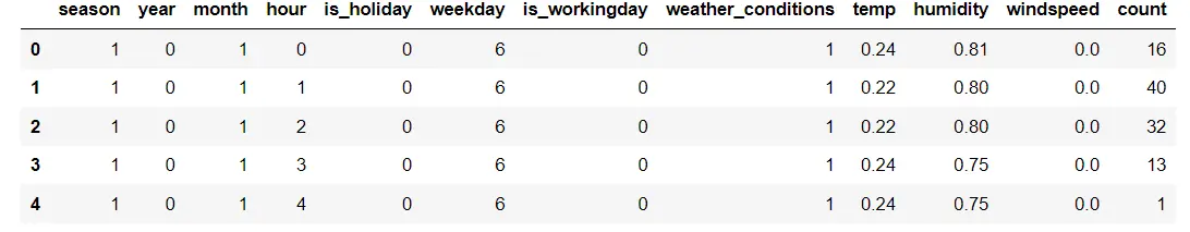
In addition, we will exclude the 'datetime' column from our dataset. With the data cleaning process now finished, we can train our model.

First, we define our features (X) and target variable (Y). The dataset is then split into training and test sets using the train_test_split() function from scikit-learn.

The split is performed in a ratio of 80% for training data and 20% for testing data. This division effectively allows us to evaluate our model's performance on unseen data.

data.drop(['datetime'], axis = 1, inplace = True)
Y = data['count']
X = data.drop('count', axis = 1)
X_train, X_test, Y_train, Y_test = train_test_split(X, Y, test_size = 0.20)

Model Selection and Training

For the model selection part, we try 2 different models, which include:

1. Linear Regression Model.
2. Random Forest Regressor.

We train the model of our dataset and then select one based on models performance. The metric used in our case is root mean squared error.

1. Linear Regression

Linear regression is a statistical model fitting a linear equation to a dataset to minimize the difference between the observed and predicted values.

The goal is to find the best coefficients (w1, ..., wp) that minimize the sum of squared differences between the actual and predicted values.

The linear regression model approximates the relationship between the input and target variables by finding the line that best fits the data points.

Below attached is the code for using Linear regression on our dataset. As we have performed the regression task, we have used root mean squared error as the loss function.

model = LinearRegression()
model.fit(X_train, Y_train)
pred = model.predict(X_test)
mse = sklearn.metrics.mean_squared_error(Y_test, pred)
rmse = math.sqrt(mse)
print(rmse)

137.39450694606478

2. Random Forest Regressor

The random forest algorithm is a powerful method for classification tasks. It involves creating multiple decision trees on different subsets of the dataset and combining their predictions to improve accuracy and prevent overfitting.

The size of each subset can be controlled using the max_samples parameter. By default, the algorithm uses bootstrap sampling, which means each subset is created by randomly selecting data points with replacements from the original dataset.

model_2 = RandomForestRegressor(n_estimators = 200, max_depth = 15)
model_2.fit(X_train, Y_train)
pred = model_2.predict(X_test)
mse = sklearn.metrics.mean_squared_error(Y_test, pred)
rmse = math.sqrt(mse)
rmse

43.7065261288683

Since the random forest regression model exhibits a lower root mean squared error (RMSE) value, it can be considered a superior model to linear regression.

Hence, we will employ the random forest regression model to construct the machine learning pipeline.

Creating an ML Pipeline for Prediction

Scikit-learn offers convenient pipeline creation functions, namely sklearn.pipeline and sklearn.make_pipeline. These functions simplify the construction of pipelines by providing streamlined implementations.

You can refer to the documentation to learn more about make_pipeline and explore all the parameters of the sklearn.pipeline.

In the following code, we construct a pipeline based on the data and steps we previously worked on:

1. Load the data.
2. Perform data preprocessing.
3. Split the data.
4. Apply transformations to the data using the fit() method.
5. Finally, predict the output on the test set and evaluate the performance of the model.
   

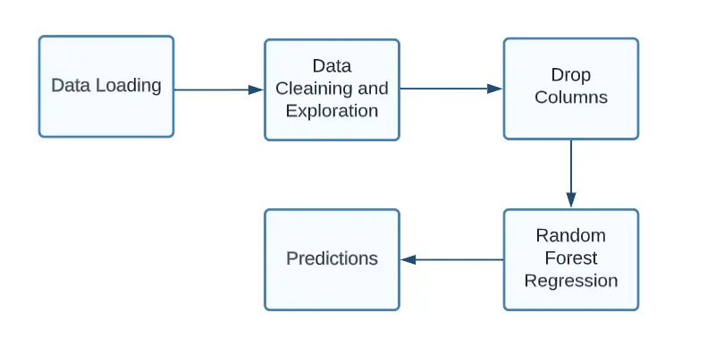
   Figure: Flowchart Pipeline for our model (Image by author)

To create an end-to-end pipeline, we import Pipeline, which is provided via the scikit-learn package.

from sklearn.ensemble import RandomForestRegressor
from sklearn.model_selection import train_test_split
from sklearn.metrics import mean_squared_error
from sklearn.pipeline import Pipeline

pipeline = Pipeline(steps = [
('model',model_2)
])

model = pipeline.fit(X_train, y_train)
predictions = pipeline.predict(X_test)
print(math.sqrt(sklearn.metrics.mean_squared_error(Y_test, predictions)))

43.7065261288683

Conclusion

In conclusion, building an end-to-end machine learning pipeline is crucial for effectively and efficiently implementing machine learning models. It automates and standardizes the workflow, ensuring reproducibility and simplifying orchestration.

The benefits of having an end-to-end pipeline include ensuring reproducibility, simplifying orchestration, accelerating deployment, enabling focus on innovation, and facilitating the reusability of components.

In the process of building a machine learning pipeline, data exploration and preprocessing play a significant role. It involves tasks such as loading the data, handling missing values, renaming columns, converting data types, and addressing multicollinearity.

After preprocessing the data, we train and evaluate different models. In the example, we used linear regression and random forest regression models. The model with the lower root mean squared error (RMSE) is considered superior.

To simplify the pipeline construction, scikit-learn provides functions like sklearn.pipeline and sklearn.make_pipeline. These functions allow for the easy creation of pipelines with various data transformations and model training steps.

Finally, we create the machine learning pipeline by loading the data, performing preprocessing, splitting the data, applying transformations using the fit() method, and making predictions to evaluate the model's performance.

Frequently Asked Questions (FAQ)

What is an End-to-End Machine Learning Pipeline?

An end-to-end machine learning pipeline automates machine learning workflow by handling data processing, integration, model creation, evaluation, and delivery. It streamlines the implementation of the model and enhances its flexibility.

What are the fundamental stages in an ML pipeline?

Stages of a Machine Learning Pipeline

1. Data Preprocessing. The initial stage of any pipeline involves data preprocessing. ...
2. Data Cleaning. Following data preprocessing, the data proceeds to the cleaning stage.
3. Feature Engineering.
4. Model Selection.
5. Prediction Generation.

What are the various categories of ML pipelines?

ML pipelines can be categorized into two main types: Transformer and Estimator. A Transformer operates on a dataset and generates an enhanced version of the dataset as output. For example, a tokenizer is a Transformer that converts a text dataset into a dataset with tokenized words.