How self driving cars predict the motion of pixels in frames, explained!

Autonomous vehicles have been a long-awaited dream for so many of us in artificial intelligence. About 30 years ago, Dickmanns and Zapp integrated several classical computer vision algorithms in a system that would drive their car automatically on a highway, and ever since that the technology has been growing.

Autonomous vehicles need to be able to perceive both the presence and motion of objects in the surrounding environment to navigate in the real world.

For this, autonomous vehicles receive and have to process sensory information coming from the surrounding world. A major sensory input is vision and it is a challenge to extract all the relevant information from road image sequences acquired by a camera mounted on the autonomous vehicle.

The vision systems of these vehicles are focused on the detection of those features necessary to control the steering position and the detection of obstacles. The control of self-driving cars has received growing attention recently.

Motion detection is a fundamental but challenging task for autonomous driving. Self-driving cars use optical flow networks to estimate the motion of objects on the road. This is later used for making decisions to control the car.

Motion estimation, that too in real-time, is very important for realizing a self-driving car as we need to predict the motion of other objects surrounding the car well in advance to predict & avoid possible collisions, adjust the speed of the vehicle and achieve safe driving, just like we humans do when we drive.

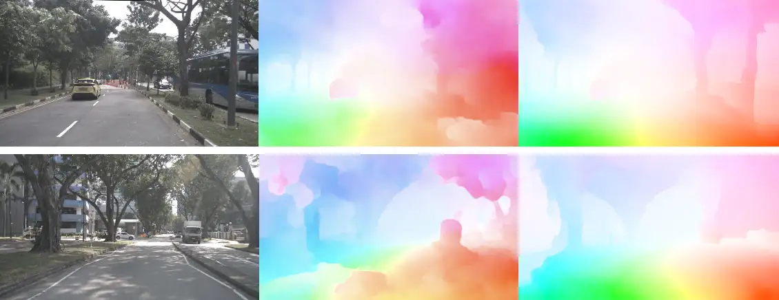
Img: Optical Flow in Autonomous Vehicles

Introduction

Recent breakthroughs in computer vision research have allowed machines to perceive its surrounding world through techniques such as object detection for detecting instances of objects belonging to a certain class and image segmentation for pixel-wise classification.

We have talked more about object detection and image segmentation in our other blogs.  A complete guide on object detection & its use in self-driving cars

However, for processing real-time video input, most implementations of these techniques only address relationships of objects within the same frame, disregarding time information. In other words, they evaluate each frame independently, as if they are completely unrelated images, for each run.

However, what if we do need the relationships between consecutive frames, for example, we want to track the motion of vehicles across frames to estimate their current velocity and predict their position in the next frame?

The solution to this is Optical Flow. Optical flow is defined as the two-dimensional motion of pixels or objects between two images. In simple words, we can track and predict the motion of pixels or objects among various frames using Optical Flow. You can see an example of this in the image below.

Img: Optical Flow

Optical flow provides essential information about the scene and serves as input for several tasks such as ego-motion estimation and object tracking.

You can read more about ego-motion estimation and object tracking in our other blogs. (Links)

Hence, optical flow is one building block of a self-driving system, just like depth estimation, object detection, and so on.

You can learn more here: Object Scene Flow for Autonomous Vehicles Object Scene Flow for Autonomous Vehicles

Let us start by understanding what Optical Flow actually is.

What is Optical flow?

Optical flow or optic flow is the pattern of apparent motion of objects or individual pixels in a visual scene caused by the relative motion between an observer and a scene.

In simple words, Optical flow is the pattern of motion of objects between two consecutive frames caused by the movement of an object or camera, or both.

It is a 2D vector field where each vector is a displacement vector showing the movement of points or pixels) from the first frame to the second.

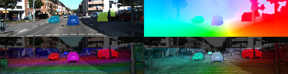
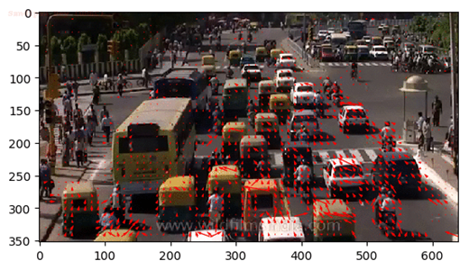
For example, in a traffic scene, Optical Flow will show the motion of cars or pedestrians between two consecutive frames. To show this, generally, displacement vectors (or arrows) are used which will point towards the direction of movement of the object (or feature) they represent. Sometimes, the length of the arrow may represent the velocity of the object or feature.

You can learn more here: Optical Flow - Computerphile Overview | Optical Flow Optical Flow in Computer Vision

We can also see a similar example in the image below where the optical flow of a traffic scene is shown and each arrow points in the direction of the predicted flow of the corresponding pixel.

Img: Optical Flow of Traffic

To predict (or calculate) the position or speed in the next frame, generally the change in position of the pixel (or feature) or object in the last two frames is observed with respect to time.

Generally, there are two types of Optical Flow :

1. Sparse Optical Flow: Sparse optical flow gives the flow vectors of some "features" (say few pixels depicting the edges or corners of an object) within the frame.
2. Dense Optical Flow: Dense optical flow, gives the flow vectors of the entire frame (all pixels) - up to one flow vector per pixel. Dense optical flow has higher accuracy at the cost of being slow/computationally expensive.

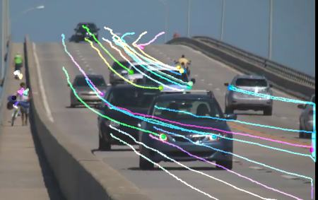
In simple words, during Sparse Optical Flow only some pixels that we also refer to as features are passed to the Optical flow function, while all pixels are passed to the Optical Flow function during Dense Optical Flow. We can clearly see the difference in both in the image below, where Sparse Optical Flow - which tracks a few "feature" pixels is shown on the left, and Dense Optical Flow - which estimates the flow of all pixels in the image, is shown in the right.

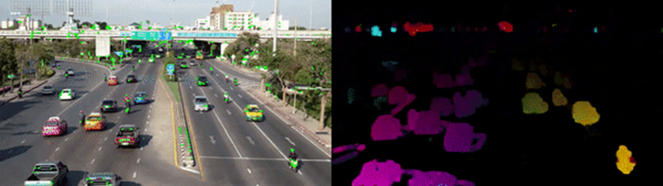
Img: Sparse Optical Flow (Left) vs Dense Optical Flow (Right)

There may be scenarios where you want to only track a specific object of interest (say tracking a certain person) or one category of objects (like all 2 wheeler-vehicles in traffic). We can combine Object Detection with this Optical Flow method to only estimate the flow of pixels within the detected bounding boxes. This way we can track all objects of a particular type/category in the video.

Let us now try to understand how Optical Flow is achieved.

How is Optical flow achieved?

Optical flow works on several assumptions:

• The pixel intensities of an object do not change between consecutive frames.
• Neighboring pixels have similar motions.

Generally, the optical flow of a pixel is calculated using the optical flow equation.

Consider a pixel I(x,y,t) in the first frame. It moves by distance (dx,dy) in the next frame taken after time dt. So since those pixels are the same and intensity does not change, we can say,

I(x,y,t)=I(x+dx,y+dy,t+dt)

From this, we can obtain the optical flow equation by first taking taylor series approximation of the right-hand side, then removing common terms and finally dividing by dt. We’ll get the following equation:

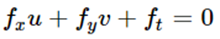
The above equation is called the Optical Flow equation, where:

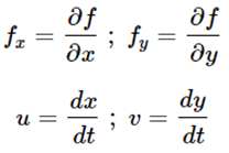
Here, fx and fy are image gradients. Similarly, ft is the gradient over time. But (u,v) are unknowns. We cannot solve this one equation with two unknown variables. So several methods are provided to solve this problem and one of them is Lucas-Kanade. Let us discuss it briefly.

Lucas-Kanade method

We have seen an assumption before, that all the neighboring pixels will have similar motion. The Lucas-Kanade method takes a 3x3 patch of pixels around the point (pixel). So all the 9 points have the same motion.

We can find (fx, fy, ft) for these 9 points. So now our problem becomes solving 9 equations with two unknown variables which are over-determined.

Below is the final solution which is two equations-two unknown problems that can be solved to get the solution.

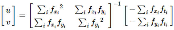
This is all the mathematical processing going on in the program to calculate the optical flow of a pixel using the optical flow equation. But, from the user's point of view, the idea is simple: we give some points to track, and we receive the optical flow vectors of those points.

You can learn more here: Optical Flow Constraint Equation | Optical Flow Lucas-Kanade Method | Optical Flow

But, despite the long history of the optical flow problem, occlusions, large displacement, and fine details are still challenging for modern methods.

Nowadays, many end-to-end deep learning models like Flow-Net, SpyNet, and PWC-Net are available, which give great accuracy in real-time. But, a big problem that remains for deep learning models is the limited amount of training data, which is not able to cover all scenarios.

Another fundamental problem with the optical flow definition is that besides the actual motion of interest, illumination changes, reflections, and transparency can also cause intensity changes.

Also, it is easier to deal with small motions, but most optical flow algorithms fail when there is a large motion.

Summary

Optical flow can be obtained from road image sequences. From this optical flow, relevant information for road navigation can be obtained.

Fundamentally, optical flow vectors function as input to many higher-level tasks requiring scene understanding of video sequences while these tasks may further act as building blocks to yet more complex systems such as facial expression analysis, autonomous vehicle navigation, and much more.

Robust optical flow methods need to handle intensity changes not caused by the actual motion of interest but by illumination changes, reflections, and transparency.

In real-world scenes, repetitive patterns, texture-less surfaces, saturated image regions, and occlusions are frequent sources of errors. These problems mostly remain mostly unsolved.

Reflective, and transparent regions also result in large errors in many cases. A better understanding of the world is necessary to tackle these problems.

A highly accurate and very fast optical flow algorithm is necessary to build an autonomous vehicle. Still, there is a lot of scope for research in this field.

Although, it is completely true that technology is growing very rapidly and we may see fully autonomous vehicles on roads sooner than expected.