
Micro-Organism Image Classification Using Deep Learning: ML Experts Guide
Guide to micro-organism image classification using deep learning, detailing data prep, model building, training, and real-world applications in disease diagnosis, drug discovery, and ecology

Introduction
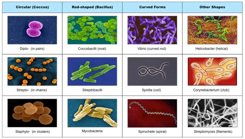
Microscopic creatures, like bacteria and tiny organisms, play big roles in science. In fields like health and technology, telling these small creatures apart using pictures is super important for finding diseases, making new medicines, and understanding the environment.
This guide helps explain how to build a really smart computer model that can spot and categorize these tiny beings in pictures. It breaks down each step, making it easier for anyone interested, whether you're a beginner or an expert, to explore this tiny world.
From getting the pictures ready to using them in real-life tasks, every part of this guide shows how important it is to use computers to understand these tiny but powerful living things, highlighting how technology can help us learn more and make new discoveries in science.
Use Cases in Life Sciences and Biotechnology
Micro-organism image classification has various applications in the life sciences and biotechnology industries. It aids in:
Disease Identification: Assisting in identifying diseases caused by specific micro-organisms.
Drug Development: Supporting drug discovery by understanding the behavior of different micro-organisms and their response to drugs.
Environmental Studies: Facilitating environmental monitoring by identifying beneficial or harmful micro-organisms in different ecosystems.
Accurate classification of micro-organisms through deep learning models enhances research, diagnostics, and applications in these fields.
Hands-on Tutorial
(1) Importing Libraries and Dataset
The initial step involves importing necessary libraries such as Pandas, NumPy, Matplotlib, TensorFlow, and Keras, among others. These libraries provide functions and tools for data manipulation, visualization, and deep learning.
import os,glob
import pandas as pd
import numpy as np
import matplotlib.pyplot as plt
from sklearn.model_selection import train_test_split
from random import randint
from keras.preprocessing.image import ImageDataGenerator
import tensorflow as tf
from tensorflow.keras.applications import VGG16
from tensorflow.keras.layers import Dense, GlobalAveragePooling2D
from tensorflow.keras.layers import Input
from tensorflow.keras.models import Model
from tensorflow.keras.callbacks import Callback,EarlyStopping
from tensorflow.keras.preprocessing.image import img_to_array,load_img
from sklearn.metrics import classification_report
import numpy as np
from os import path, listdir
(2) Exploring and Loading the Dataset
The dataset containing images of various micro-organisms is loaded and prepared for analysis. It consists of images belonging to 8 different classes of micro-organisms.
# Specify root path
root_path = '../input/microorganism-image-classification/Micro_Organism/'
name_class = os.listdir(root_path)
dataset_Path = list(glob.glob(root_path+'/**/*.*'))
labels = list(map(lambda x : os.path.split(os.path.split(x)[0])[1],dataset_Path))
dataset_Path = pd.Series(dataset_Path,name = 'FilePath').astype(str)
labels = pd.Series(labels,name='Label')
data = pd.concat([dataset_Path,labels],axis =1)
data = data.sample(frac=1).reset_index(drop= True)
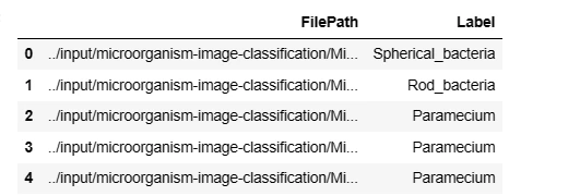
data.head(5)This code section involves loading the dataset, creating file paths, extracting labels, and organizing the data into a Pandas DataFrame for further analysis.
(3) Data Visualization
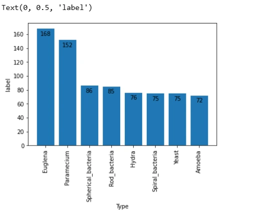
Understanding the class distribution within the dataset is essential. Visualizing the distribution of classes using a bar plot helps identify potential class imbalances.
def addlabels(x,y):
    for i in range(len(x)):
        plt.text(i,y[i]-10,y[i], ha = 'center')

counts = data.Label.value_counts()

plt.bar(counts.index, counts)
addlabels(counts.index, counts)
plt.xticks(rotation=90)
plt.xlabel('Type')
plt.ylabel('label')
This snippet generates a bar plot displaying the number of images in each class, facilitating an understanding of the dataset's distribution.
fig,axes = plt.subplots(nrows=5,ncols=3,figsize=(10,8),subplot_kw={'xticks':[],'yticks':[]})
for i ,ax,in enumerate(axes.flat):
  ax.imshow(plt.imread(data.FilePath[i]))
  ax.set_title(data.Label[i])
plt.tight_layout()
plt.show()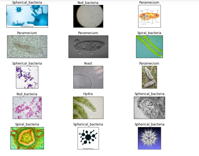
(4) Data Splitting and Augmentation
Preparing the dataset for training involves resizing images to a uniform size and applying augmentation techniques such as flipping and rotation to increase the dataset's diversity.
train,rem = train_test_split(data,test_size =0.20,random_state = 42 )
test,valid = train_test_split(data,test_size =0.50,random_state = 42 )

train_datagen = ImageDataGenerator(
    horizontal_flip=True,
    vertical_flip=True,
    rotation_range=10,
)
test_datagen = ImageDataGenerator()
train_gen = train_datagen.flow_from_dataframe(dataframe = train,x_col = 'FilePath',
y_col = 'Label',target_size=(224,224), class_mode ='categorical',
color_mode='rgb',batch_size =8,shuffle = True,seed =42)
valid_gen = train_datagen.flow_from_dataframe(dataframe = valid,x_col = 'FilePath',
y_col = 'Label',target_size=(224,224), class_mode ='categorical',
color_mode='rgb',batch_size =8,shuffle = False,seed =42)
test_gen = test_datagen.flow_from_dataframe(dataframe = test,x_col = 'FilePath',
y_col = 'Label',target_size=(224,224), class_mode ='categorical',
color_mode='rgb',batch_size =8,shuffle = False,seed =42)This snippet performs the actual split of the dataset into training, validation, and test sets. It uses flow_from_dataframe method from Keras' ImageDataGenerator to generate batches of augmented image data, specifying parameters like target size, color mode, batch size, and more.
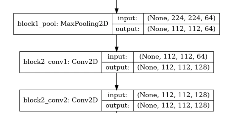
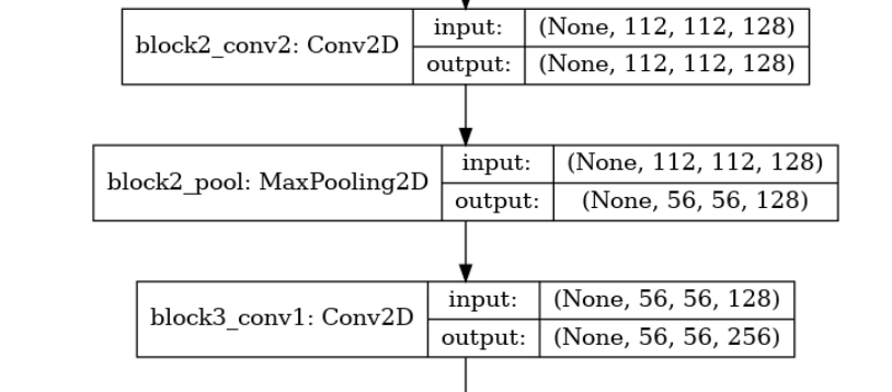
(5) Building the Model (Transfer Learning with VGG16)
In this section, the VGG16 model without its top classification layers is utilized as a base model. Additional dense layers are added on top of the base model to improve classification performance. The Model class from Keras is used to construct the final model architecture.
NO_CLASSES = max(train_gen.class_indices.values()) + 1
base_model = VGG16(include_top=False, input_shape=(224, 224, 3))

x = base_model.output
x = GlobalAveragePooling2D()(x) #used to replace fully connected layers in classical CNNs.
#It will generate one feature map for each corresponding category of the
classification task in the last mlpcov layer(1 X 1 convolutions).
x = Dense(1024,activation='relu')(x)   # add dense layers so learn
more complex functions and classify for better results.
x = Dense(1024,activation='relu')(x)   # dense layer 2
x = Dense(512,activation='relu')(x)    # dense layer 3

preds = Dense(NO_CLASSES,activation='softmax')(x)
model = Model(inputs = base_model.input, outputs = preds) #create a new model with
the base model's original input
Here in VGG16, include_top is false because we want to add more dense layers. Most models are a series of convolutional layers followed by one or a few dense (or fully connected) layers. include_top Help us select the last dense layer or not.
Convolution layers act as feature extractors.They identiy a series of patterns in the image ,and each layer can identify more elborate patterns by seeing patterns of patterns. The dense layes are capable of interpreting the found patterns in order to classify the image of various categories.
(6) Freezing and Fine-Tuning Model Layers
This code snippet freezes the first 19 layers of the model (the convolutional base) to retain the previously learned features and fine-tunes the remaining layers for improved accuracy in identifying micro-organisms' distinct features.
#don't train the first 19 layers
for layer in model.layers[:19]:
    layer.trainable=False
#train the rest of the layers
for layer in model.layers[19:]:
    layer.trainable=True
(7) Plotting Model Architecture
tf.keras.utils.plot_model(model,'model.png',show_shapes=True)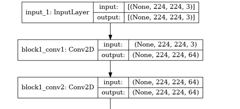
(8) Compiling and Training the Model
This section involves compiling the model with an optimizer, specifying the loss function and metrics. The fit method is used to train the model using the prepared training data and validation data while employing early stopping callbacks for monitoring the validation accuracy.
#Compiling Model
model.compile(optimizer='Adam',loss='categorical_crossentropy',metrics=['accuracy'])

#callbacks
my_callbacks = [EarlyStopping(monitor = 'val_accuracy',min_delta=0,patience=2,mode='auto')]

model.fit(train_gen,validation_data = valid_gen,
          epochs=25,callbacks=[my_callbacks])
(9) Evaluating the Model and Making Predictions
The evaluate method is used to assess the model's performance on the test set, providing information about the loss and accuracy metrics. This step helps in understanding how well the trained model generalizes to unseen data.
model.evaluate(test_gen)(10) Generating Predictions and Classification Report
Here, the code utilizes the trained model to predict classes for the test dataset. The predict method generates predictions, and then, the results are converted back to class labels using the dictionary created earlier. The classification_report function from sklearn computes and displays precision, recall, F1-score, and support for each class, providing insights into the model's performance.
#predict the label of the test_gen
pred = model.predict(test_gen)
pred = np.argmax(pred,axis=1)
labels = (train_gen.class_indices)
labels = dict((v,k) for k,v, in labels.items()) #
pred = [labels[k]for k in pred]
y_test = list(test.Label)
print(classification_report(y_test,pred))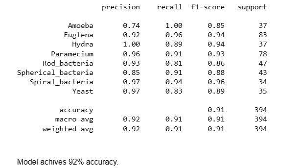
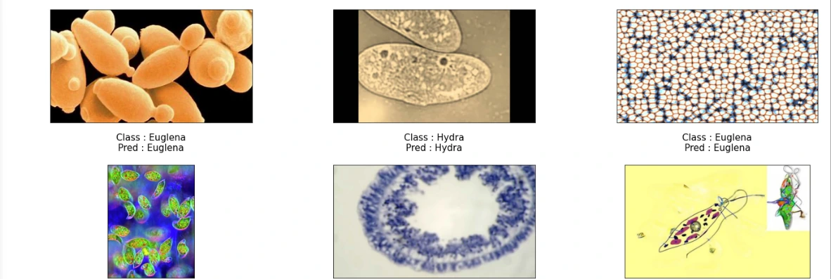
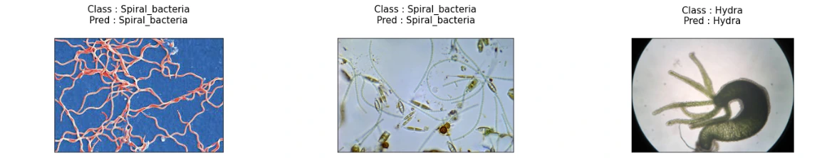
(11) Storing Class Labels and Visualization of Model Predictions
This snippet maps class indices to their respective labels for better interpretation. Subsequently, it visualizes the model's predictions on sample images from the test set, displaying both the true class and the predicted class for each image.
labels = (train_gen.class_indices)

pred = model.predict(test_gen)
pred = np.argmax(pred,axis=1)
labels = dict((v,k) for k,v, in labels.items())
pred = [labels[k]for k in pred]

fig,axes = plt.subplots(nrows=5,ncols=3,figsize=(20,18),subplot_kw={'xticks':[],'yticks':[]})
for i ,ax,in enumerate(axes.flat):
    ax.imshow(plt.imread(test_gen.filenames[i]))
    title =str( f"Class : {labels[test_gen.classes[i]]}\nPred : {pred[i]}\n")
    ax.set_title(title,fontsize=15)
plt.tight_layout()
plt.show()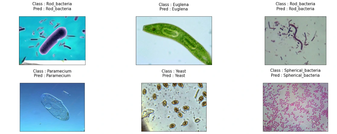
With Labellerr's SaaS data annotation platform, you can effortlessly label and prepare high-quality datasets for deep learning models. Accelerate your research by using our platform. Sign up today. Book a Demo
Conclusion
This comprehensive tutorial walks through the complete process of micro-organism image classification using deep learning. It covers data preprocessing, model building, training, evaluation, and real-world applications in life sciences and biotechnology.
Understanding and accurately classifying micro-organisms through image classification models can significantly impact research, diagnostics, and various industries, facilitating advancements in disease identification, drug development, and environmental studies.
Frequently Asked Questions
1. Can deep learning be used to analyze microorganisms based on human-operated microscopy?
Deep learning methodologies have been suggested as a solution to address the difficulties encountered in human-operated microscopy. These methods are aimed at analyzing microscopic images of various microorganisms, such as viruses, bacteria, fungi, and parasites.
2. How ML techniques are used in bacterial image classification?
Machine learning (ML) techniques are pivotal in bacterial image classification, leveraging algorithms like convolutional neural networks (CNNs) to discern intricate patterns within images. Through supervised learning, these models are trained on extensive datasets, learning to differentiate between various bacterial species based on visual features. Transfer learning, where pre-trained models are adapted and fine-tuned on specific bacterial datasets, accelerates this process by utilizing knowledge from prior tasks. These ML techniques enable automated and accurate identification of bacteria, aiding in disease diagnosis, drug development, and environmental analysis, revolutionizing research and applications in microbiology.
3. What are the applications of deep-learning-based microscopic image analysis?
Deep learning finds widespread application in microscopic image analysis, primarily in image classification, detection, and segmentation. Image classification discerns between infected and uninfected samples viewed under a microscope. Object detection seeks to pinpoint the presence and location of infected cells within the image.

Simplify Your Data Annotation Workflow With Proven Strategies
.png)