Breast Cancer Detection Model: Tutorial to Analyze Mammography Images

Introduction

Breast cancer remains a significant health concern globally, but advancements in medical imaging technology and machine learning offer promising avenues for early detection and diagnosis.

Mammography, a standard imaging technique, coupled with deep learning models, presents a powerful tool for identifying breast abnormalities, thereby aiding medical professionals in timely interventions and treatments.

In this tutorial, we will walk through a comprehensive Python guide that covers various aspects of processing mammography images, cleaning and preparing datasets, building a Convolutional Neural Network (CNN) model, and making predictions for breast cancer detection.

Hands-on Tutorial

Outline

(i) Understanding the Dataset

(ii) Data Preprocessing and Cleaning

(iii) Exploratory Data Analysis (EDA)

(iv) Image Visualization and Insights

(v) Building a Convolutional Neural Network (CNN) Model

(vi) Training and Evaluating the CNN Model

(vii) Predictions and Model Deployment

1. Understanding the Dataset

Pandas Import: The code imports the Pandas library, a powerful tool for data manipulation and analysis.

Reading Dataset: It reads the breast cancer image dataset from a CSV file using Pandas' read_csv function.

Exploring Dataset: The .head() function displays the first few rows of the dataset, giving an overview of its structure, while .info() provides information about columns and data types.

import os
from os import listdir
import pandas as pd 
import numpy as np 
import matplotlib.pyplot as plt 
import plotly.express as px
import seaborn as sns

import cv2
from matplotlib.image import imread

import tensorflow as tf
from keras.utils.np_utils import to_categorical
from keras.preprocessing import image
from sklearn.model_selection import train_test_split
from sklearn.metrics import confusion_matrix


import glob
import PIL
import random

random.seed(100)

dicom_data = pd.read_csv('/kaggle/input/cbis-ddsm-breast-cancer-image-dataset/csv/dicom_info.csv')
image_dir = '/kaggle/input/cbis-ddsm-breast-cancer-image-dataset/jpeg'

dicom_data.head()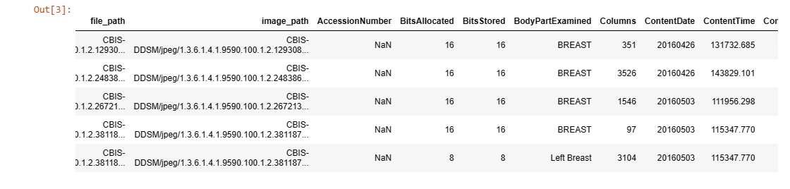

dicom_data.info()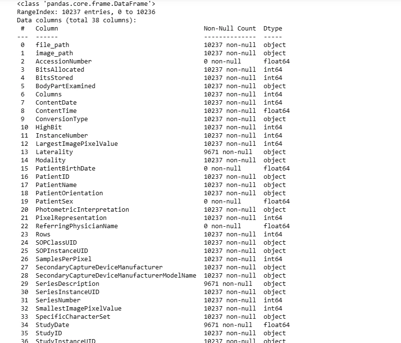

cropped_images = dicom_data[dicom_data.SeriesDescription == 'cropped images'].image_path
cropped_images.head()

cropped_images = cropped_images.apply(lambda x: x.replace('CBIS-DDSM/jpeg', image_dir))
cropped_images.head()

for file in cropped_images[0:10]:
    cropped_images_show = PIL.Image.open(file)
    gray_img= cropped_images_show.convert("L")
    plt.imshow(gray_img, cmap='gray')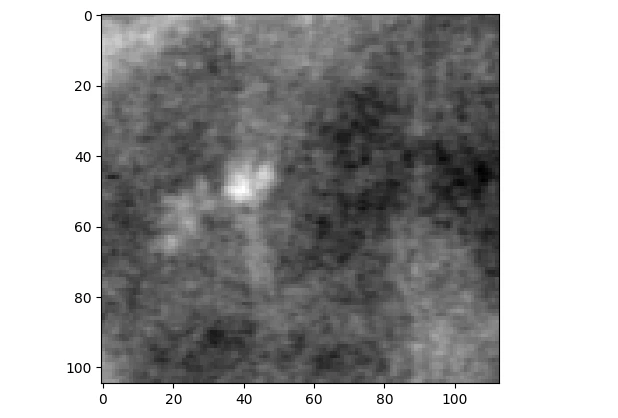

full_mammogram_images = dicom_data[dicom_data.SeriesDescription == 'full mammogram images'].image_path
full_mammogram_images.head()

full_mammogram_images = full_mammogram_images.apply(lambda x: x.replace('CBIS-DDSM/jpeg', image_dir))
full_mammogram_images.head()

for file  in full_mammogram_images[0:10]:
    full_mammogram_images_show = PIL.Image.open(file)
    gray_img= full_mammogram_images_show.convert("L")
    plt.imshow(gray_img, cmap='gray')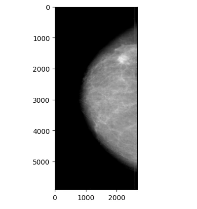

ROI_mask_images = dicom_data[dicom_data.SeriesDescription == 'ROI mask images'].image_path
ROI_mask_images.head()

ROI_mask_images = ROI_mask_images.apply(lambda x: x.replace('CBIS-DDSM/jpeg', image_dir))
ROI_mask_images.head()

for file  in ROI_mask_images[0:10]:
    ROI_mask_images_show = PIL.Image.open(file)
    gray_img= ROI_mask_images_show.convert("L")
    plt.imshow(gray_img, cmap='gray')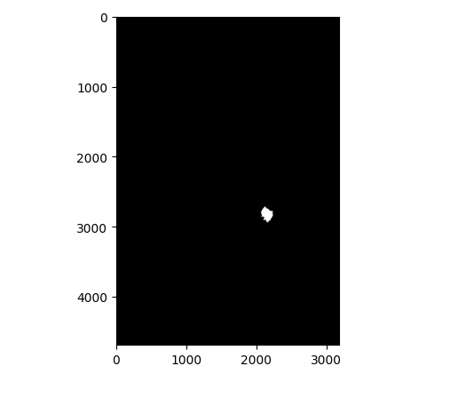

calc_case_df = pd.read_csv('/kaggle/input/cbis-ddsm-breast-cancer-image-dataset/csv/calc_case_description_train_set.csv')

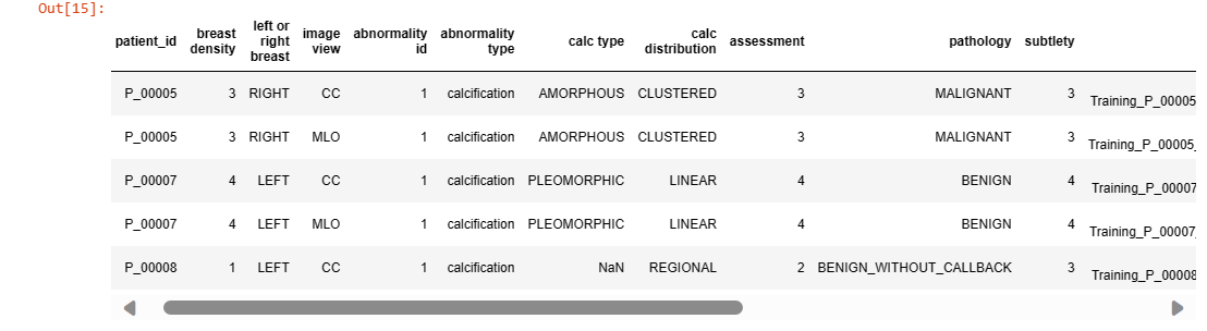
calc_case_df.head(5)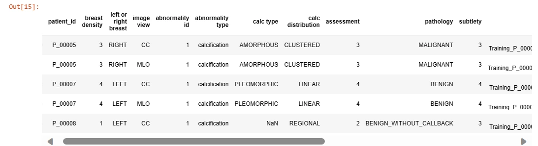

mass_case_df = pd.read_csv('/kaggle/input/cbis-ddsm-breast-cancer-image-dataset/csv/mass_case_description_train_set.csv')

mass_case_df.head(5)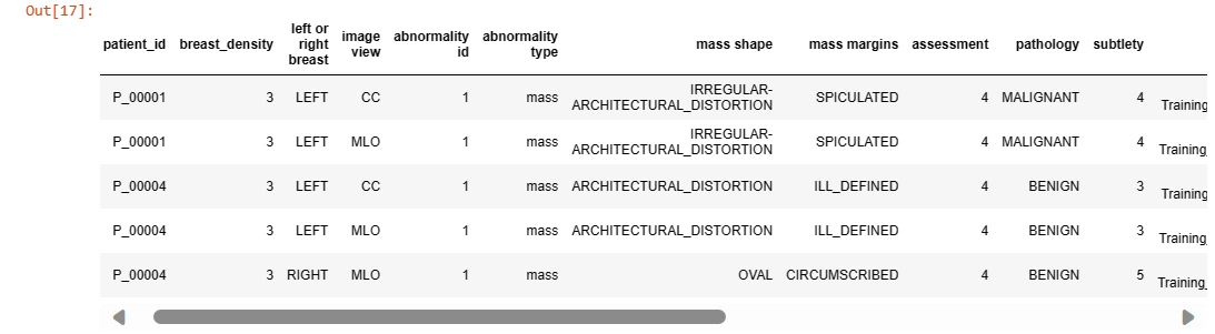

Understanding the dataset's structure is crucial before diving into analysis. It includes information such as image paths, patient details, and metadata required for preprocessing and analysis.

2. Data Preprocessing and Cleaning

Copying Data: Creates a copy of the dataset to retain the original dataset for reference.

Handling Missing Values: Uses Pandas' fillna method to handle missing values in the 'SeriesDescription' column by backfilling missing values with the next available value.

data_insight_2 = pd.DataFrame({'abnormality':[Data_cleaning_1.abnormality_type[0],Data_cleaning_2.abnormality_type[0]],

dicom_cleaned_data.drop(['PatientBirthDate','AccessionNumber','Columns','ContentDate','ContentTime','PatientSex','PatientBirthDate',
                                                'ReferringPhysicianName','Rows','SOPClassUID','SOPInstanceUID',
                                                'StudyDate','StudyID','StudyInstanceUID','StudyTime','InstanceNumber','SeriesInstanceUID','SeriesNumber'],axis =1, inplace=True) 
                                                
dicom_cleaned_data.info()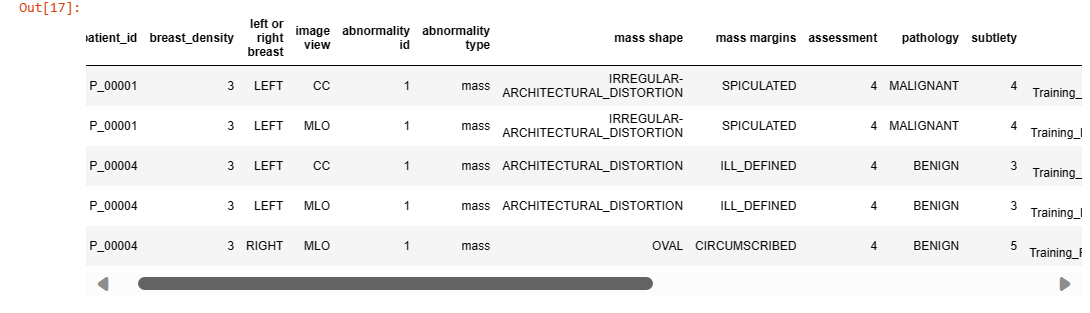

dicom_cleaned_data.isna().sum()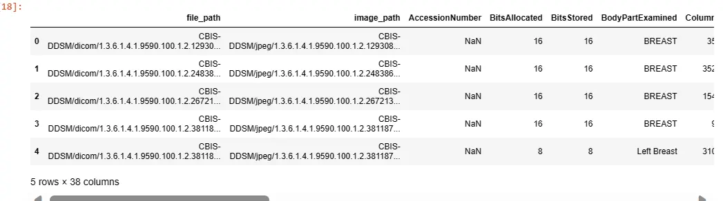

dicom_cleaned_data['SeriesDescription'].fillna(method = 'bfill', axis = 0, inplace=True)

dicom_cleaned_data['Laterality'].fillna(method = 'bfill', axis = 0, inplace=True)

dicom_cleaned_data.isna().sum()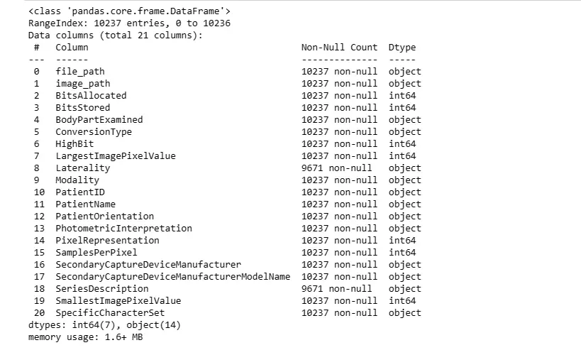

Data_cleaning_1 = calc_case_df.copy()
Data_cleaning_1 = Data_cleaning_1.rename(columns={'calc type':'calc_type'})
Data_cleaning_1 = Data_cleaning_1.rename(columns={'calc distribution':'calc_distribution'})
Data_cleaning_1 = Data_cleaning_1.rename(columns={'image view':'image_view'})
Data_cleaning_1 = Data_cleaning_1.rename(columns={'left or right breast':'left_or_right_breast'})
Data_cleaning_1 = Data_cleaning_1.rename(columns={'breast density':'breast_density'})
Data_cleaning_1 = Data_cleaning_1.rename(columns={'abnormality type':'abnormality_type'})
Data_cleaning_1['pathology'] = Data_cleaning_1['pathology'].astype('category')
Data_cleaning_1['calc_type'] = Data_cleaning_1['calc_type'].astype('category')
Data_cleaning_1['calc_distribution'] = Data_cleaning_1['calc_distribution'].astype('category')
Data_cleaning_1['abnormality_type'] = Data_cleaning_1['abnormality_type'].astype('category')
Data_cleaning_1['image_view'] = Data_cleaning_1['image_view'].astype('category')
Data_cleaning_1['left_or_right_breast'] = Data_cleaning_1['left_or_right_breast'].astype('category')
Data_cleaning_1.isna().sum()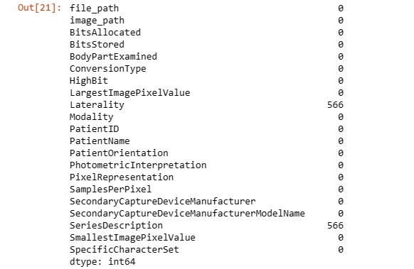

Data_cleaning_1['calc_type'].fillna(method = 'bfill', axis = 0, inplace=True) 
Data_cleaning_1['calc_distribution'].fillna(method = 'bfill', axis = 0, inplace=True)
Data_cleaning_1.isna().sum()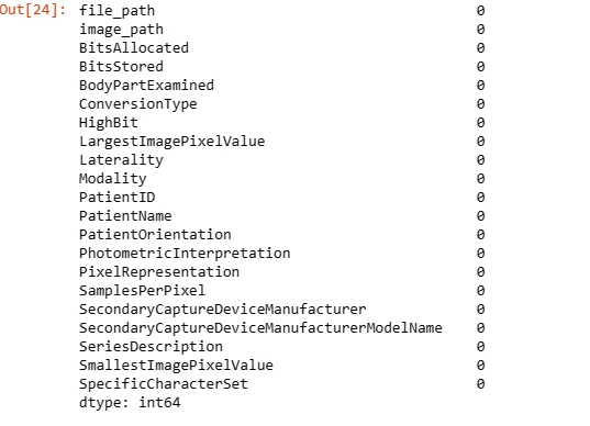

Data_cleaning_2 = mass_case_df.copy()
Data_cleaning_2 = Data_cleaning_2.rename(columns={'mass shape':'mass_shape'})
Data_cleaning_2 = Data_cleaning_2.rename(columns={'left or right breast':'left_or_right_breast'})
Data_cleaning_2 = Data_cleaning_2.rename(columns={'mass margins':'mass_margins'})
Data_cleaning_2 = Data_cleaning_2.rename(columns={'image view':'image_view'})
Data_cleaning_2 = Data_cleaning_2.rename(columns={'abnormality type':'abnormality_type'})
Data_cleaning_2['left_or_right_breast'] = Data_cleaning_2['left_or_right_breast'].astype('category')
Data_cleaning_2['image_view'] = Data_cleaning_2['image_view'].astype('category')
Data_cleaning_2['mass_margins'] = Data_cleaning_2['mass_margins'].astype('category')
Data_cleaning_2['mass_shape'] = Data_cleaning_2['mass_shape'].astype('category')
Data_cleaning_2['abnormality_type'] = Data_cleaning_2['abnormality_type'].astype('category')
Data_cleaning_2['pathology'] = Data_cleaning_2['pathology'].astype('category')
Data_cleaning_2.isna().sum()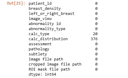

Data_cleaning_2['mass_shape'].fillna(method = 'bfill', axis = 0, inplace=True) 
Data_cleaning_2['mass_margins'].fillna(method = 'bfill', axis = 0, inplace=True) 
Data_cleaning_2.isna().sum()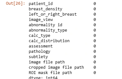

Data preprocessing involves steps like handling missing values, dropping irrelevant columns, and formatting data to ensure accuracy and consistency in subsequent analysis tasks.

3. Exploratory Data Analysis (EDA)

Data Visualization: Uses Plotly Express (plotly.express) to create a bar chart (px.bar) displaying the types of images used based on the 'SeriesDescription' column.

breast_imgs = glob.glob('/kaggle/input/breast-histopathology-images/IDC_regular_ps50_idx5/**/*.png', recursive = True)

for imgname in breast_imgs[:5]:
    print(imgname)
    
 non_cancer_imgs = []
cancer_imgs = []

for img in breast_imgs:
    if img[-5] == '0' :
        non_cancer_imgs.append(img)
    
    elif img[-5] == '1' :
        cancer_imgs.append(img)
        
non_cancer_num = len(non_cancer_imgs)  # No cancer
cancer_num = len(cancer_imgs)   # Cancer 
        
total_img_num = non_cancer_num + cancer_num
        
print('Number of Images of no cancer: {}' .format(non_cancer_num))   # images of Non cancer
print('Number of Images of cancer : {}' .format(cancer_num))   # images of cancer 
print('Total Number of Images : {}' .format(total_img_num))        

data_insight_1 = pd.DataFrame({'state of cancer' : ['0','1'],'Numbers of Patients' : [198738,78786]})

bar = px.bar(data_frame=data_insight_1, x = 'state of cancer', y='Numbers of Patients', color='state of cancer')
bar.update_layout(title_text='Number of Patients with cancer (1) and patients with no cancer (0)', title_x=0.5)
bar.show()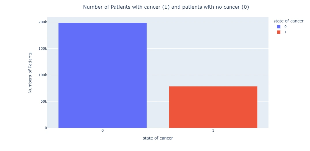

EDA aids in gaining insights into the dataset's composition, identifying patterns, and understanding the distribution of image types, which is crucial in understanding available image variations and their relevance.

4. Image Visualization and Insights

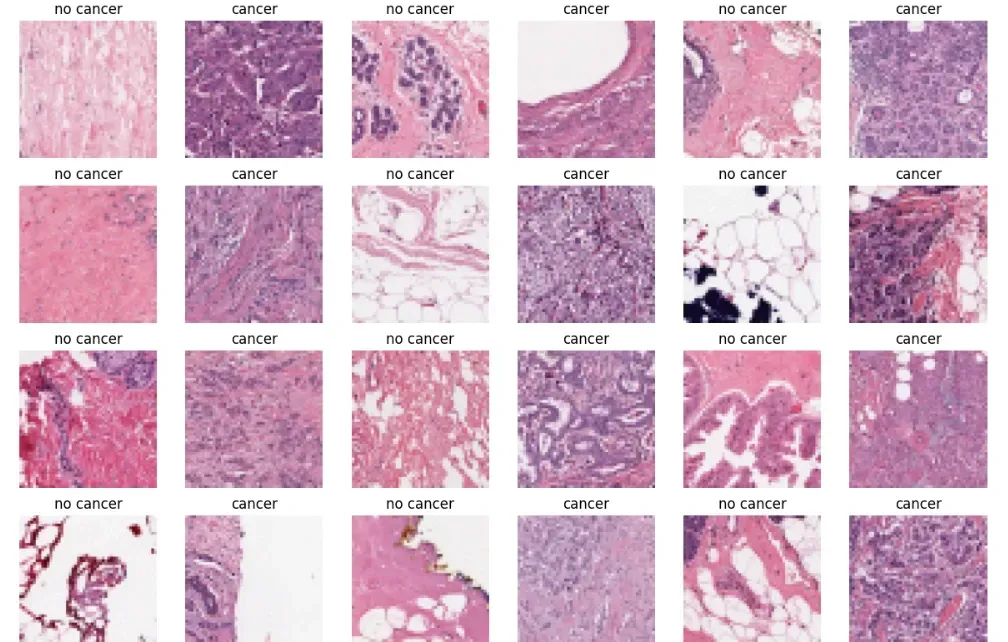
Image Visualization: Utilizes Matplotlib to display sample images from the dataset (here, 'cropped_images') in grayscale for visualization purposes.

r= pd.DataFrame(dicom_cleaned_data['SeriesDescription'].value_counts())
r= r.reset_index()
r= r.rename(columns={'SeriesDescription':'SeriesDescription_counts', 'index':'SeriesDescription'})
r

ba_1 = px.bar(data_frame=dicom_cleaned_data, x='SeriesDescription', color='SeriesDescription',
              title='Types of images used')
ba_1.update_layout(title_text='Types of images used', title_x=0.5)
ba_1.show()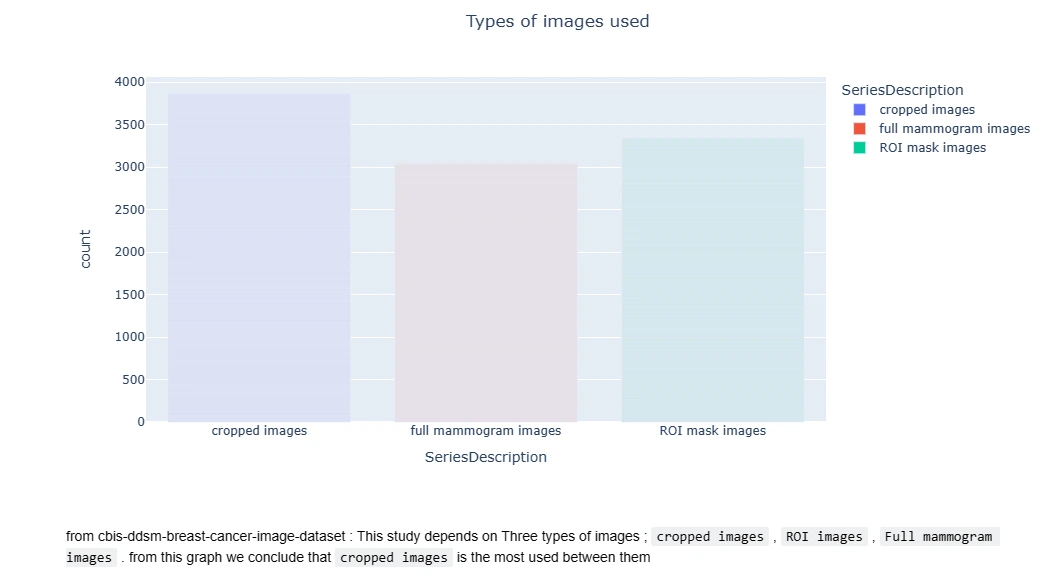

f= pd.DataFrame(dicom_cleaned_data['BodyPartExamined'].value_counts())
f= f.reset_index()
f= f.rename(columns={'BodyPartExamined':'BodyPartExamined_counts', 'index':'Breast part Examined'})
f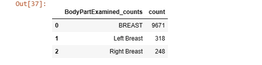

ba = px.bar(data_frame=f, x="BodyPartExamined_counts", y="count", color="BodyPartExamined_counts")
ba.update_layout(title_text='Breast Parts Examined', title_x=0.5, yaxis=dict(type='log'))
ba.show()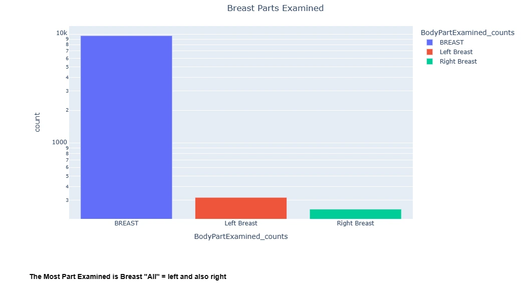

data_insight_2 = pd.DataFrame({'abnormality':[Data_cleaning_1.abnormality_type[0],Data_cleaning_2.abnormality_type[0]],
                               'counts_of_abnormalties':[len(Data_cleaning_1),len(Data_cleaning_2)]})
data_insight_2

bar_2 =px.bar(data_frame=data_insight_2, x = 'abnormality', y='counts_of_abnormalties', color = 'abnormality')
bar_2.update_layout(title_text='Types of abnormalites of cancer', title_x=0.5)
bar_2.show()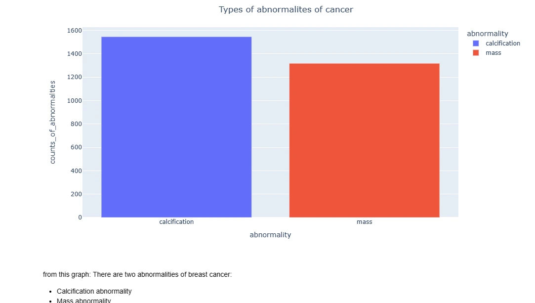

x = Data_cleaning_1.left_or_right_breast.value_counts().RIGHT
y = Data_cleaning_1.left_or_right_breast.value_counts().LEFT
print(x,y)

data_insight_3 = pd.DataFrame({'left_or_right_breast':['RIGHT','LEFT'] , 'Counts':[x,y]})
data_insight_3

insight_3 = px.bar(data_insight_3, y= 'Counts', x='left_or_right_breast',color = 'left_or_right_breast')
insight_3.update_layout(title_text=' clacification cancer position of the breasts ', title_x=0.5)
insight_3.show()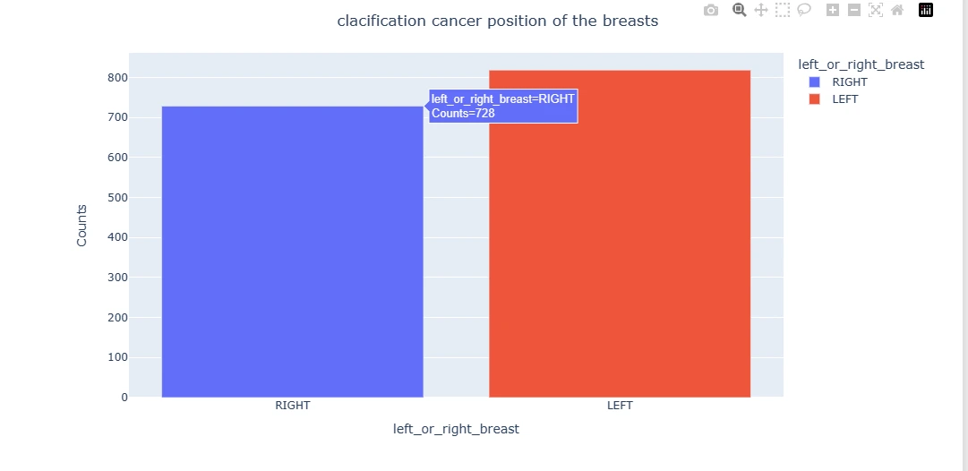

z = pd.DataFrame(Data_cleaning_1['calc_type'].value_counts())
z = z.reset_index()
z= z.rename(columns={'calc_type':'calc_type_counts'})
z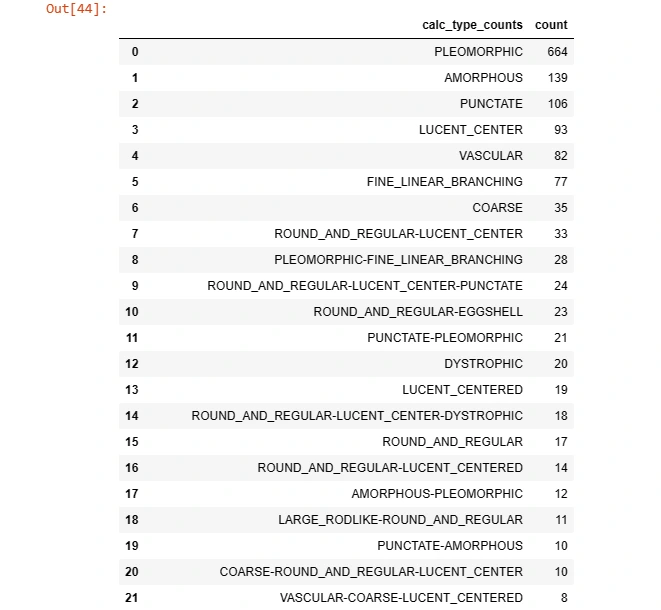

plt.figure(figsize = (15, 15))

some_non = np.random.randint(0, len(non_cancer_imgs), 18)
some_can = np.random.randint(0, len(cancer_imgs), 18)

s = 0
for num in some_non:
    
        img = image.image_utils.load_img((non_cancer_imgs[num]), target_size=(100, 100))
        img = image.image_utils.img_to_array(img)
        
        plt.subplot(6, 6, 2*s+1)
        plt.axis('off')
        plt.title('no cancer')
        plt.imshow(img.astype('uint8'))
        s += 1
        
s = 1
for num in some_can:
    
        img = image.image_utils.load_img((cancer_imgs[num]), target_size=(100, 100))
        img = image.image_utils.img_to_array(img)
        plt.subplot(6, 6, 2*s)
        plt.axis('off')        
        plt.title('cancer')
        plt.imshow(img.astype('uint8'))
        s += 1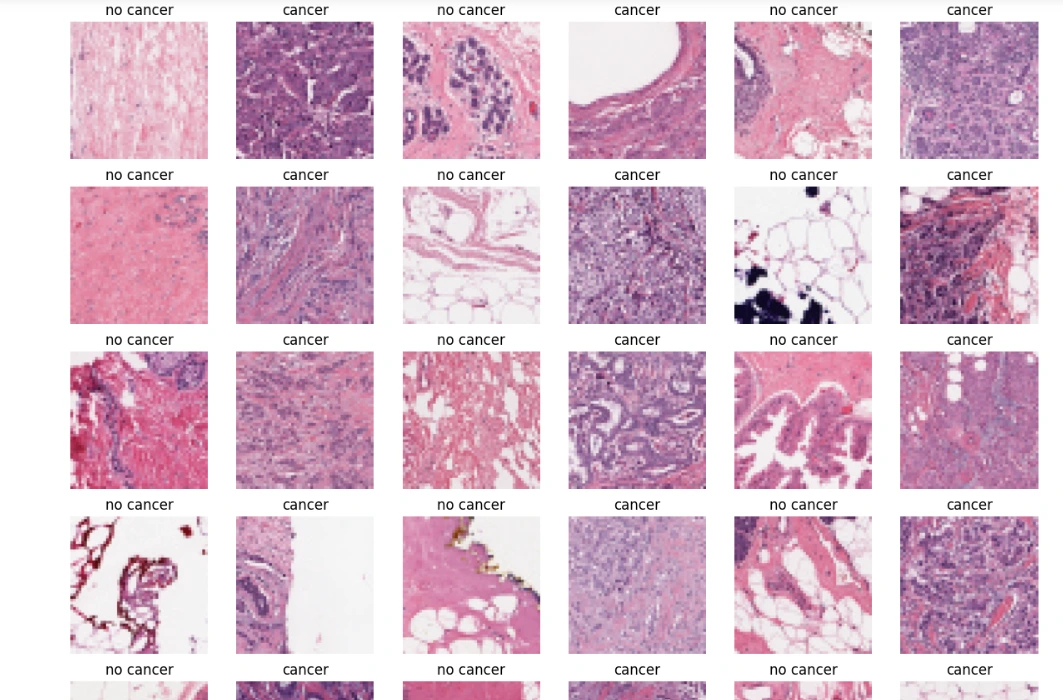

Visualizing sample images provides an overview of mammogram representations, showcasing differences and potential abnormalities present in the dataset.

5. Building a Convolutional Neural Network (CNN) Model

TensorFlow Import: Import TensorFlow, a popular deep learning framework for building neural network models.

Sequential Model: Define a sequential CNN model architecture using TensorFlow's Keras API and compile the model with an optimizer, loss function, and evaluation metric.

# Randomly sample images from two lists, 'non_cancer_imgs' and 'cancer_imgs'
some_non_img = random.sample(non_cancer_imgs, len(non_cancer_imgs))
some_can_img = random.sample(cancer_imgs, len(cancer_imgs))

# Initialize empty arrays to store image data and labels
non_img_arr = []  # Array for non-cancer images
can_img_arr = []  # Array for cancer images

# Loop through each image in the 'some_non_img' list
for img in some_non_img:
    # Read the image in color mode
    n_img = cv2.imread(img, cv2.IMREAD_COLOR)
    # Resize the image to a fixed size (50x50 pixels) using linear interpolation
    n_img_size = cv2.resize(n_img, (50, 50), interpolation=cv2.INTER_LINEAR)
    # Append the resized image and label 0 (indicating non-cancer) to the 'non_img_arr'
    non_img_arr.append([n_img_size, 0])

# Loop through each image in the 'some_can_img' list
for img in some_can_img:
    # Read the image in color mode
    c_img = cv2.imread(img, cv2.IMREAD_COLOR)
    # Resize the image to a fixed size (50x50 pixels) using linear interpolation
    c_img_size = cv2.resize(c_img, (50, 50), interpolation=cv2.INTER_LINEAR)
    # Append the resized image and label 1 (indicating cancer) to the 'can_img_arr'
    can_img_arr.append([c_img_size, 1])

X = []  # List for image data
y = []  # List for labels

# Concatenate the arrays 'non_img_arr' and 'can_img_arr' into a single array 'breast_img_arr'
breast_img_arr = np.concatenate((non_img_arr, can_img_arr))

# Shuffle the elements in the 'breast_img_arr' array randomly
random.shuffle(breast_img_arr)

# Loop through each element (feature, label) in the shuffled 'breast_img_arr'
for feature, label in breast_img_arr:
    # Append the image data (feature) to the 'X' list
    X.append(feature)
    # Append the label to the 'y' list
    y.append(label)

# Convert the lists 'X' and 'y' into NumPy arrays
X = np.array(X)
y = np.array(y)

# Print the shape of the 'X' array
print('X shape: {}'.format(X.shape))

# Split the dataset into training and testing sets, with a test size of 20%
X_train, X_test, y_train, y_test = train_test_split(X, y, test_size=0.20, random_state=42)

# Define a rate (percentage) for subsampling the training data
rate = 0.5

# Calculate the number of samples to keep in the training data based on the rate
num = int(X.shape[0] * rate)

# Convert the categorical labels in 'y_train' and 'y_test' to one-hot encoded format
y_train = to_categorical(y_train, 2)  # Assuming there are 2 classes (non-cancer and cancer)
y_test = to_categorical(y_test, 2)


print('X_train shape : {}' .format(X_train.shape))
print('X_test shape : {}' .format(X_test.shape))
print('y_train shape : {}' .format(y_train.shape))
print('y_test shape : {}' .format(y_test.shape))

from tensorflow.keras.preprocessing.image import ImageDataGenerator
# Data augmentation
datagen = ImageDataGenerator(
    rotation_range=20,
    width_shift_range=0.2,
    height_shift_range=0.2,
    shear_range=0.2,
    zoom_range=0.2,
    horizontal_flip=True,
    fill_mode='nearest'
)

# Create data generators for training and testing
train_datagen = datagen.flow(X_train, y_train, batch_size=32)
test_datagen = datagen.flow(X_test, y_test, batch_size=32, shuffle=False)

# Define an EarlyStopping callback
early_stopping = tf.keras.callbacks.EarlyStopping(
    monitor='val_loss',          # Monitor the validation loss
    patience=5,                  # Number of epochs with no improvement after which training will be stopped
    min_delta=1e-7,              # Minimum change in the monitored quantity to be considered an improvement
    restore_best_weights=True,   # Restore model weights from the epoch with the best value of monitored quantity
)

# Define a ReduceLROnPlateau callback
plateau = tf.keras.callbacks.ReduceLROnPlateau(
    monitor='val_loss',   # Monitor the validation loss
    factor=0.2,           # Factor by which the learning rate will be reduced (new_lr = lr * factor)
    patience=2,           # Number of epochs with no improvement after which learning rate will be reduced
    min_delta=1e-7,       # Minimum change in the monitored quantity to trigger a learning rate reduction
    cooldown=0,           # Number of epochs to wait before resuming normal operation after learning rate reduction
    verbose=1             # Verbosity mode (1: update messages, 0: no messages)
)

# Set a random seed for reproducibility
tf.random.set_seed(42)

# Create a Sequential model
model = tf.keras.Sequential([
    # Convolutional layer with 32 filters, a 3x3 kernel, 'same' padding, and ReLU activation
    tf.keras.layers.Conv2D(32, (3, 3), padding='same', activation='relu', input_shape=(50, 50, 3)),
    tf.keras.layers.BatchNormalization(),
    # MaxPooling layer with a 2x2 pool size and default stride (2)
    tf.keras.layers.MaxPooling2D(strides=2),
    
    # Convolutional layer with 64 filters, a 3x3 kernel, 'same' padding, and ReLU activation
    tf.keras.layers.Conv2D(64, (3, 3), padding='same', activation='relu'),
    tf.keras.layers.BatchNormalization(),
    # MaxPooling layer with a 3x3 pool size and stride of 2
    tf.keras.layers.MaxPooling2D((3, 3), strides=2),
    
    # Convolutional layer with 128 filters, a 3x3 kernel, 'same' padding, and ReLU activation
    tf.keras.layers.Conv2D(128, (3, 3), padding='same', activation='relu'),
    tf.keras.layers.BatchNormalization(),
    # MaxPooling layer with a 3x3 pool size and stride of 2
    tf.keras.layers.MaxPooling2D((3, 3), strides=2),
    
    # Convolutional layer with 128 filters, a 3x3 kernel, 'same' padding, and ReLU activation
    tf.keras.layers.Conv2D(128, (3, 3), padding='same', activation='relu'),
    tf.keras.layers.BatchNormalization(),
    # MaxPooling layer with a 3x3 pool size and stride of 2
    tf.keras.layers.MaxPooling2D((3, 3), strides=2),
    
    # Flatten the output to prepare for fully connected layers
    tf.keras.layers.Flatten(),
    
    # Fully connected layer with 128 units and ReLU activation
    tf.keras.layers.Dense(128, activation='relu'),
    tf.keras.layers.Dropout(0.3),
    # Output layer with 2 units (binary classification) and softmax activation
    tf.keras.layers.Dense(2, activation='softmax')
])

# Display a summary of the model architecture
model.summary()

# Compile the model with Adam optimizer, binary cross-entropy loss, and accuracy metric
model.compile(optimizer=tf.keras.optimizers.Adam(learning_rate=0.001),
              loss='binary_crossentropy',
              metrics=['accuracy'])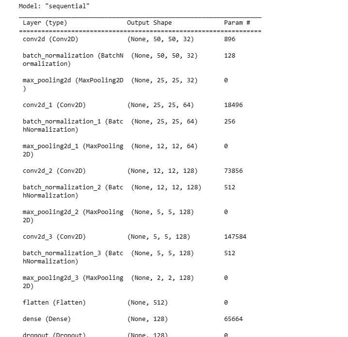

CNNs are suitable for image-based tasks due to their ability to learn features hierarchically. Building a CNN model for breast cancer detection is a fundamental step in leveraging machine learning for medical image analysis.

6. Training and Evaluating the CNN Model

Model Training: Uses the fit method to train the CNN model on training data (X_train and y_train) for a specified number of epochs and batch size.

Model Evaluation: Evaluate the trained model's performance on the test set using the evaluate method.

Training and evaluating the model help assess its performance metrics (like accuracy, and loss) on both training and unseen test data, ensuring its effectiveness in detecting breast cancer.

history = model.fit(X_train,
                    y_train,
                    validation_data = (X_test, y_test),
                    epochs = 25,
                    batch_size = 75,
                    callbacks=[early_stopping, plateau])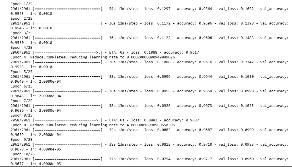

model.evaluate(X_test,y_test)

7. Predictions and Model Deployment

Making Predictions: Generate predictions using the trained CNN model on test data.

Example Prediction: Demonstrates how to make predictions on a single image by interpreting the predicted class based on the probability threshold.

Y_pred = model.predict(X_test)
Y_pred_classes = np.argmax(Y_pred,axis = 1) 
Y_true = np.argmax(y_test,axis = 1) 

confusion_mtx = confusion_matrix(Y_true, Y_pred_classes) 
f,ax = plt.subplots(figsize=(8, 8))
sns.heatmap(confusion_mtx, annot=True, linewidths=0.01,cmap="BuPu",linecolor="gray", fmt= '.1f',ax=ax)
plt.xlabel("Predicted Label")
plt.ylabel("True Label")
plt.title("Confusion Matrix")
plt.show()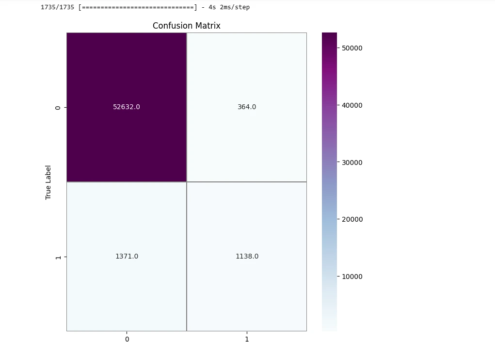

plt.plot(history.history['accuracy'])
plt.plot(history.history['val_accuracy'])
plt.title('Model Accuracy')
plt.ylabel('accuracy')
plt.xlabel('epoch')
plt.legend(['train', 'test'], loc='upper left')
plt.show()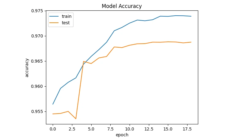

plt.plot(history.history['loss'])
plt.plot(history.history['val_loss'])
plt.title('Model Loss')
plt.ylabel('loss')
plt.xlabel('epoch')
plt.legend(['train', 'test'], loc='upper left')
plt.show()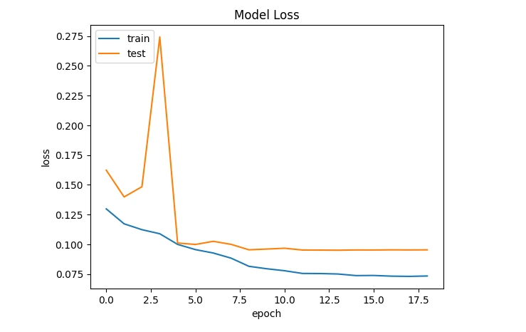

prediction = model.predict(X_test)
prediction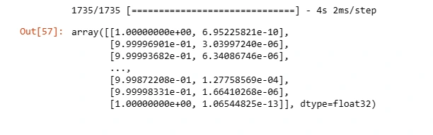

Making predictions and understanding the model's output is crucial in practical deployment scenarios for diagnosing breast cancer based on mammography images.

8. Testing Model

# Define a mapping of class indices to human-readable labels
class_labels = {
    0: 'Non-Cancerous',
    1: 'Cancerous',
}

# Define a mapping of calcification types
calcification_types = {
    0: 'No Calcification',
    1: 'PLEOMORPHIC',
    2: 'AMORPHOUS',
    3: 'PUNCTATE',
    4: 'LUCENT_CENTER',
    5: 'VASCULAR',
    6: 'FINE_LINEAR_BRANCHING',
    7: 'COARSE',
    8: 'ROUND_AND_REGULAR-LUCENT_CENTER',
    9: 'PLEOMORPHIC-FINE_LINEAR_BRANCHING',
    10: 'ROUND_AND_REGULAR-LUCENT_CENTER-PUNCTATE',
    11: 'ROUND_AND_REGULAR-EGGSHELL',
    12: 'PUNCTATE-PLEOMORPHIC',
    13: 'DYSTROPHIC',
    14: 'LUCENT_CENTERED',
    15: 'ROUND_AND_REGULAR-LUCENT_CENTER-DYSTROPHIC',
    16: 'ROUND_AND_REGULAR',
    17: 'ROUND_AND_REGULAR-LUCENT_CENTERED',
    18: 'AMORPHOUS-PLEOMORPHIC',
    19: 'LARGE_RODLIKE-ROUND_AND_REGULAR',
    20: 'PUNCTATE-AMORPHOUS',
    21: 'COARSE-ROUND_AND_REGULAR-LUCENT_CENTER',
    22: 'VASCULAR-COARSE-LUCENT_CENTERED',
    23: 'LUCENT_CENTER-PUNCTATE',
    24: 'ROUND_AND_REGULAR-PLEOMORPHIC',
    25: 'EGGSHELL',
    26: 'PUNCTATE-FINE_LINEAR_BRANCHING',
    27: 'VASCULAR-COARSE',
    28: 'ROUND_AND_REGULAR-PUNCTATE',
    29: 'SKIN-PUNCTATE-ROUND_AND_REGULAR',
    30: 'SKIN-PUNCTATE',
    31: 'COARSE-ROUND_AND_REGULAR-LUCENT_CENTERED',
    32: 'PUNCTATE-ROUND_AND_REGULAR',
    33: 'LARGE_RODLIKE',
    34: 'AMORPHOUS-ROUND_AND_REGULAR',
    35: 'PUNCTATE-LUCENT_CENTER',
    36: 'SKIN',
    37: 'VASCULAR-COARSE-LUCENT_CENTER-ROUND_AND_REGULA',
    38: 'COARSE-PLEOMORPHIC',
    39: 'ROUND_AND_REGULAR-PUNCTATE-AMORPHOUS',
    40: 'COARSE-LUCENT_CENTER',
    41: 'MILK_OF_CALCIUM',
    42: 'COARSE-ROUND_AND_REGULAR',
    43: 'SKIN-COARSE-ROUND_AND_REGULAR',
    44: 'ROUND_AND_REGULAR-AMORPHOUS',
    45: 'PLEOMORPHIC-PLEOMORPHIC'
}

# Define a function for plotting an image from an array
def img_plot(arr, index=0):
    # Set the title for the plot
    plt.title('Test Image')
    
    # Display the image at the specified index in the array
    plt.imshow(arr[index])

# Set the index value to 90
index = 90

# Plot an image from the X_test array using the img_plot function
img_plot(X_test, index)

# Extract a single image from X_test based on the specified index
input = X_test[index:index+1]

# Make a prediction using the CNN model and get the class with the highest probability
predicted_class_index = model.predict(input)[0].argmax()

# Get the true label from the y_test array
true_class_index = y_test[index].argmax()

# Get the predicted and true labels
predicted_label = class_labels[predicted_class_index]
true_label = class_labels[true_class_index]

# Get the calcification type based on the predicted class index (modify as needed)
calcification_type = calcification_types[predicted_class_index]

# Print the prediction result with calcification type
print('Predicted Diagnosis:', predicted_label)
print('Calcification Type:', calcification_type)
print('True Diagnosis:', true_label)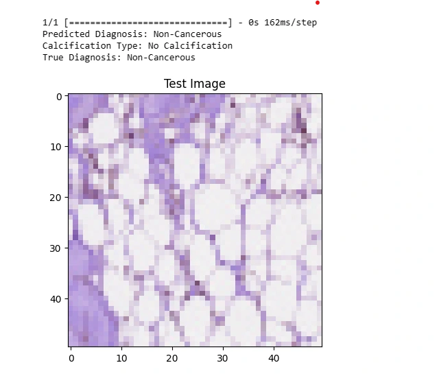

# Directory containing the images
imgs_dir = glob.glob('/kaggle/input/miniddsm2/MINI-DDSM-Complete-JPEG-8/Benign/**/*.jpeg', recursive=True)

# Example image path
image_path = '/kaggle/input/miniddsm2/MINI-DDSM-Complete-JPEG-8/Benign/0029/C_0029_1.LEFT_CC.jpg'

# Define a function to load and preprocess an image
def load_and_preprocess_image(image_path, target_size=(50, 50)):
    try:
        # Load and preprocess the image
        img = cv2.imread(image_path)
        img = cv2.cvtColor(img, cv2.COLOR_BGR2RGB)  # Convert BGR to RGB format
        img = cv2.resize(img, target_size)  # Resize to your target size
        img_array = img / 255.0  # Normalize pixel values

        return img_array
    except Exception as e:
        print(f"Error processing {image_path}: {str(e)}")
        return None

# Load and preprocess the example image
img_array = load_and_preprocess_image(image_path)

if img_array is not None:
    # Create a batch for prediction (even if it's a single image)
    img_batch = np.expand_dims(img_array, axis=0)

    # Make predictions
    predictions = model.predict(img_batch)

    # Assuming your model predicts binary probabilities, you can get the probability for "Cancer" class
    cancer_probability = predictions[0][0]  # Assuming "Cancer" is the first class

    # Get the predicted class label
    predicted_class = "Cancer" if cancer_probability >= 0.5 else "Normal"

    # Plot the image and display the predicted class and probability
    plt.imshow(img)
    plt.title(f'Predicted Class: {predicted_class}\nProbability of Cancer: {cancer_probability:.4f}')
    plt.axis('off')
    plt.show()
else:
    print("Image loading and preprocessing failed.")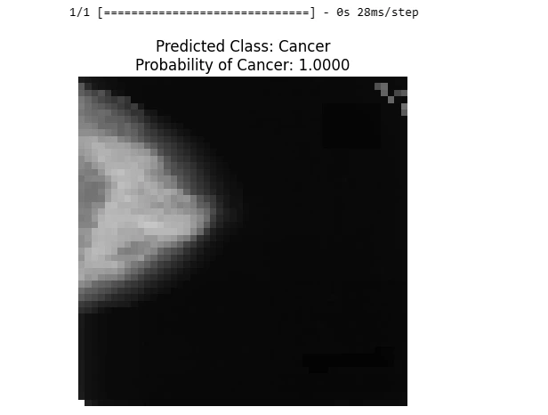

Use Cases in the Medical and Healthcare Industry

Early Detection: Automated detection systems aid in identifying potential abnormalities at an early stage, improving patient outcomes and treatment options.

Treatment Planning: Accurate identification of abnormalities assists medical professionals in devising effective treatment plans tailored to individual patient needs.

Research and Development: Large-scale datasets and machine learning facilitate ongoing research, leading to innovations and advancements in breast cancer diagnosis and treatment.

Frequently Asked Questions

1. How is CNN used for breast cancer detection?

Convolutional Neural Networks (CNNs) are instrumental in breast cancer detection by analyzing mammography images. These networks excel in recognizing intricate patterns and features within medical images, crucial for identifying abnormalities indicative of breast cancer.

CNNs process these images through numerous convolutional and pooling layers, learning hierarchical representations that capture varying complexities. By leveraging CNNs' ability to extract intricate visual patterns, healthcare professionals can accurately interpret mammograms, aiding in early detection, precise diagnosis, and personalized treatment strategies for breast cancer patients.

2. Can MobileNet detect breast cancer?

MobileNet's focus on computational efficiency enables the extraction of features from mammography images, facilitating the identification of subtle patterns or abnormalities linked to breast cancer.

This architecture proves effective in capturing crucial image details, aiding in the detection of minute indicators or irregularities associated with the disease.

3. How to detect breast cancer in mammography images?

Detecting breast cancer in mammography images involves employing CNN models to identify cancer and analyzing texture characteristics in a two-phase approach, merging the results to make a conclusive determination about cancer presence.